Read in catalog information from a text file and plot some parameters

Authors

Adrian Price-Whelan, Kelle Cruz, Stephanie T. Douglas

Learning Goals

• Read an ASCII file using astropy.io

• Convert between representations of coordinate components using astropy.coordinates (hours to degrees)

• Make a spherical projection sky plot using matplotlib

Keywords

file input/output, coordinates, tables, units, scatter plots, matplotlib

Summary

This tutorial demonstrates the use of astropy.io.ascii for reading ASCII data, astropy.coordinates and astropy.units for converting RA (as a sexagesimal angle) to decimal degrees, and matplotlib for making a color-magnitude diagram and on-sky locations in a Mollweide projection.

import numpy as np

# Set up matplotlib
import matplotlib.pyplot as plt

%matplotlib inline

Astropy provides functionality for reading in and manipulating tabular data through the astropy.table subpackage. An additional set of tools for reading and writing ASCII data are provided with the astropy.io.ascii subpackage, but fundamentally use the classes and methods implemented in astropy.table.

We’ll start by importing the ascii subpackage:

from astropy.io import ascii

For many cases, it is sufficient to use the ascii.read('filename') function as a black box for reading data from table-formatted text files. By default, this function will try to figure out how your data is formatted/delimited (by default, guess=True). For example, if your data are:

# name,ra,dec
BLG100,17:51:00.0,-29:59:48
BLG101,17:53:40.2,-29:49:52
BLG102,17:56:20.2,-29:30:51
BLG103,17:56:20.2,-30:06:22
...

(see simple_table.csv)

ascii.read() will return a Table object:

tbl = ascii.read("simple_table.csv")
tbl

Table length=4

name	ra	dec
str6	str10	str9
BLG100	17:51:00.0	-29:59:48
BLG101	17:53:40.2	-29:49:52
BLG102	17:56:20.2	-29:30:51
BLG103	17:56:20.2	-30:06:22

The header names are automatically parsed from the top of the file, and the delimiter is inferred from the rest of the file – awesome! We can access the columns directly from their names as ‘keys’ of the table object:

tbl["ra"]

<Column name='ra' dtype='str10' length=4>

17:51:00.0

17:53:40.2

17:56:20.2

17:56:20.2

If we want to then convert the first RA (as a sexagesimal angle) to decimal degrees, for example, we can pluck out the first (0th) item in the column and use the coordinates subpackage to parse the string:

import astropy.coordinates as coord
import astropy.units as u

first_row = tbl[0]  # get the first (0th) row
ra = coord.Angle(first_row["ra"], unit=u.hour)  # create an Angle object
ra.degree  # convert to degrees

np.float64(267.75)

Now let’s look at a case where this breaks, and we have to specify some more options to the read() function. Our data may look a bit messier::

,,,,2MASS Photometry,,,,,,WISE Photometry,,,,,,,,Spectra,,,,Astrometry,,,,,,,,,,,
Name,Designation,RA,Dec,Jmag,J_unc,Hmag,H_unc,Kmag,K_unc,W1,W1_unc,W2,W2_unc,W3,W3_unc,W4,W4_unc,Spectral Type,Spectra (FITS),Opt Spec Refs,NIR Spec Refs,pm_ra (mas),pm_ra_unc,pm_dec (mas),pm_dec_unc,pi (mas),pi_unc,radial velocity (km/s),rv_unc,Astrometry Refs,Discovery Refs,Group/Age,Note
,00 04 02.84 -64 10 35.6,1.01201,-64.18,15.79,0.07,14.83,0.07,14.01,0.05,13.37,0.03,12.94,0.03,12.18,0.24,9.16,null,L1γ,,Kirkpatrick et al. 2010,,,,,,,,,,,Kirkpatrick et al. 2010,,
PC 0025+04,00 27 41.97 +05 03 41.7,6.92489,5.06,16.19,0.09,15.29,0.10,14.96,0.12,14.62,0.04,14.14,0.05,12.24,null,8.89,null,M9.5β,,Mould et al. 1994,,0.0105,0.0004,-0.0008,0.0003,,,,,Faherty et al. 2009,Schneider et al. 1991,,,00 32 55.84 -44 05 05.8,8.23267,-44.08,14.78,0.04,13.86,0.03,13.27,0.04,12.82,0.03,12.49,0.03,11.73,0.19,9.29,null,L0γ,,Cruz et al. 2009,,0.1178,0.0043,-0.0916,0.0043,38.4,4.8,,,Faherty et al. 2012,Reid et al. 2008,,
...

(see Young-Objects-Compilation.csv)

If we try to just use ascii.read() on this data, it fails to parse the names out and the column names become col followed by the number of the column:

tbl = ascii.read("Young-Objects-Compilation.csv")
tbl.colnames

['col1',
 'col2',
 'col3',
 'col4',
 'col5',
 'col6',
 'col7',
 'col8',
 'col9',
 'col10',
 'col11',
 'col12',
 'col13',
 'col14',
 'col15',
 'col16',
 'col17',
 'col18',
 'col19',
 'col20',
 'col21',
 'col22',
 'col23',
 'col24',
 'col25',
 'col26',
 'col27',
 'col28',
 'col29',
 'col30',
 'col31',
 'col32',
 'col33',
 'col34']

What happened? The column names are just col1, col2, etc., the default names if ascii.read() is unable to parse out column names. We know it failed to read the column names, but also notice that the first row of data are strings – something else went wrong!

tbl[0]

Row index=0

col1	col2	col3	col4	col5	col6	col7	col8	col9	col10	col11	col12	col13	col14	col15	col16	col17	col18	col19	col20	col21	col22	col23	col24	col25	col26	col27	col28	col29	col30	col31	col32	col33	col34
str24	str25	str9	str6	str16	str5	str5	str5	str5	str5	str15	str6	str5	str6	str5	str6	str4	str6	str13	str14	str26	str23	str11	str9	str12	str10	str8	str6	str22	str6	str19	str23	str9	str38
--	--	--	--	2MASS Photometry	--	--	--	--	--	WISE Photometry	--	--	--	--	--	--	--	Spectra	--	--	--	Astrometry	--	--	--	--	--	--	--	--	--	--	--

A few things are causing problems here. First, there are two header lines in the file and the header lines are not denoted by comment characters. The first line is actually some meta data that we don’t care about, so we want to skip it. We can get around this problem by specifying the header_start keyword to the ascii.read() function. This keyword argument specifies the index of the row in the text file to read the column names from:

tbl = ascii.read("Young-Objects-Compilation.csv", header_start=1)
tbl.colnames

['Name',
 'Designation',
 'RA',
 'Dec',
 'Jmag',
 'J_unc',
 'Hmag',
 'H_unc',
 'Kmag',
 'K_unc',
 'W1',
 'W1_unc',
 'W2',
 'W2_unc',
 'W3',
 'W3_unc',
 'W4',
 'W4_unc',
 'Spectral Type',
 'Spectra (FITS)',
 'Opt Spec Refs',
 'NIR Spec Refs',
 'pm_ra (mas)',
 'pm_ra_unc',
 'pm_dec (mas)',
 'pm_dec_unc',
 'pi (mas)',
 'pi_unc',
 'radial velocity (km/s)',
 'rv_unc',
 'Astrometry Refs',
 'Discovery Refs',
 'Group/Age',
 'Note']

Great! Now the columns have the correct names, but there is still a problem: all of the columns have string data types, and the column names are still included as a row in the table. This is because by default the data are assumed to start on the second row (index=1). We can specify data_start=2 to tell the reader that the data in this file actually start on the 3rd (index=2) row:

tbl = ascii.read("Young-Objects-Compilation.csv", header_start=1, data_start=2)

Some of the columns have missing data, for example, some of the RA values are missing (denoted by – when printed):

print(tbl["RA"])

    RA   
---------
  1.01201
  6.92489
  8.23267
  9.42942
 11.33929
       --
       --
       --
 21.19163
  21.5275
      ...
       --
303.46467
   321.71
       --
       --
332.05679
333.43715
342.47273
       --
350.72079
Length = 64 rows

This is called a Masked column because some missing values are masked out upon display. If we want to use this numeric data, we have to tell astropy what to fill the missing values with. We can do this with the .filled() method. For example, to fill all of the missing values with NaN’s:

tbl["RA"].filled(np.nan)

<Column name='RA' dtype='float64' length=64>

1.01201
6.92489
8.23267
9.42942
11.33929
nan
nan
nan
21.19163
21.5275
25.49263
nan
...
300.20171
nan
303.46467
321.71
nan
nan
332.05679
333.43715
342.47273
nan
350.72079

Let’s recap what we’ve done so far, then make some plots with the data. Our data file has an extra line above the column names, so we use the header_start keyword to tell it to start from line 1 instead of line 0 (remember Python is 0-indexed!). We then used had to specify that the data starts on line 2 using the data_start keyword. Finally, we note some columns have missing values.

data = ascii.read("Young-Objects-Compilation.csv", header_start=1, data_start=2)

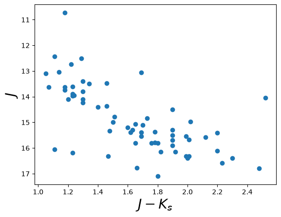
Now that we have our data loaded, let’s plot a color-magnitude diagram.

Here we simply make a scatter plot of the J-K color on the x-axis against the J magnitude on the y-axis. We use a trick to flip the y-axis plt.ylim(reversed(plt.ylim())). Called with no arguments, plt.ylim() will return a tuple with the axis bounds, e.g. (0,10). Calling the function with arguments will set the limits of the axis, so we simply set the limits to be the reverse of whatever they were before. Using this matplotlib-style plotting is convenient for making quick plots and interactive use, but is not great if you need more control over your figures.

plt.scatter(data["Jmag"] - data["Kmag"], data["Jmag"])  # plot J-K vs. J
plt.ylim(reversed(plt.ylim()))  # flip the y-axis
plt.xlabel("$J-K_s$", fontsize=20)
plt.ylabel("$J$", fontsize=20)

Text(0, 0.5, '$J$')

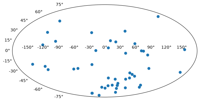
As a final example, we will plot the angular positions from the catalog on a 2D projection of the sky. Instead of using matplotlib-style plotting, we’ll take a more object-oriented approach. We’ll start by creating a Figure object and adding a single subplot to the figure. We can specify a projection with the projection keyword; in this example we will use a Mollweide projection. Unfortunately, it is highly non-trivial to make the matplotlib projection defined this way follow the celestial convention of longitude/RA increasing to the left.

The axis object, ax, knows to expect angular coordinate values. An important fact is that it expects the values to be in radians, and it expects the azimuthal angle values to be between (-180º,180º). This is (currently) not customizable, so we have to coerce our RA data to conform to these rules! astropy provides a coordinate class for handling angular values, astropy.coordinates.Angle. We can convert our column of RA values to radians, and wrap the angle bounds using this class.

ra = coord.Angle(data["RA"].filled(np.nan) * u.degree)
ra = ra.wrap_at(180 * u.degree)
dec = coord.Angle(data["Dec"].filled(np.nan) * u.degree)

fig = plt.figure(figsize=(8, 6))
ax = fig.add_subplot(111, projection="mollweide")
ax.scatter(ra.radian, dec.radian)

<matplotlib.collections.PathCollection at 0x7f3bd7be8c80>

By default, matplotlib will add degree tick labels, so let’s change the horizontal (x) tick labels to be in units of hours, and display a grid:

fig = plt.figure(figsize=(8, 6))
ax = fig.add_subplot(111, projection="mollweide")
ax.scatter(ra.radian, dec.radian)
ax.set_xticklabels(
    ["14h", "16h", "18h", "20h", "22h", "0h", "2h", "4h", "6h", "8h", "10h"]
)
ax.grid(True)

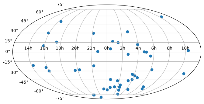
We can save this figure as a PDF using the savefig function:

fig.savefig("map.pdf")

Exercises

Make the map figures as just above, but color the points by the 'Kmag' column of the table.

Try making the maps again, but with each of the following projections: aitoff, hammer, lambert, and None (which is the same as not giving any projection). Do any of them make the data seem easier to understand?