Learn.Astropy / Tutorials

Download

Outline

1. Authors
2. Learning Goals
3. Keywords
4. Summary
   1. Imports
   2. Fit an emission line in a stellar spectrum
      1. Now that we have the spectrum...
5. Fit an Emission Line with a Gaussian Model
6. Exercise

Modeling 2: Create a User Defined Model using astropy.modeling

Authors

Rocio Kiman, Lia Corrales, Zé Vinícius, Stephanie T. Douglas

Learning Goals

• Define a new model with astropy
• Identify cases were a user-defined model could be useful
• Define models in two different ways:
  • Compound models
  • Custom models

This tutorial assumes the student knows how to fit data using astropy.modeling. This topic is covered in the Models-Quick-Fit tutorial.

Keywords

modeling, FITS, astrostatistics, matplotlib, model fitting, error bars, scatter plots

Summary

In this tutorial, we will learn how to define a new model in two ways: with a compound model and with a custom model.

with open('requirements.txt') as f:
    print(f"Required packages for this notebook:\n{f.read()}")

Required packages for this notebook:
astropy
astroquery>=0.4.8.dev9474  # 2024-09-24 pinned for Gaia column capitalization issue
matplotlib
numpy

Note: This tutorial assumes you have already gone through Modeling 1, which provides an introduction to astropy.modeling

Imports

import numpy as np
import matplotlib.pyplot as plt
from astropy.io import fits
from astropy.modeling import models, fitting
from astropy.modeling.models import custom_model
from astropy.modeling import Fittable1DModel, Parameter
from astroquery.sdss import SDSS

Fit an emission line in a stellar spectrum

M dwarfs are low mass stars (less than half of the mass of the sun). Currently we do not understand completely the physics inside low mass stars because they do not behave the same way higher mass stars do. For example, they stay magnetically active longer than higher mass stars. One way to measure magnetic activity is the height of the $H\alpha$ emission line. It is located at $6563$ Angstroms at the spectrum.

Let's search for a spectrum of an M dwarf in the Sloan Digital Sky Survey (SDSS). First, we are going to look for the spectrum in the SDSS database. SDSS has a particular way to identify the stars it observes: it uses three numbers: Plate, Fiber and MJD (Modified Julian Date). The star we are going to use has:

• Plate: 1349
• Fiber: 216
• MJD: 52797

So go ahead, put this numbers in the website and click on Plot to visualize the spectrum. Try to localize the $H\alpha$ line.

We could download the spectrum by hand from this website, but we are going to import it using the SDSSClass from astroquery.sdss. We can get the spectrum using the plate, fiber and mjd in the following way:

spectrum = SDSS.get_spectra(plate=1349, fiberID=216, mjd=52797)[0]

Now that we have the spectrum...

One way to check what is inside the fits file spectrum is the following:

spectrum[1].columns

ColDefs(
    name = 'flux'; format = 'E'
    name = 'loglam'; format = 'E'
    name = 'ivar'; format = 'E'
    name = 'and_mask'; format = 'J'
    name = 'or_mask'; format = 'J'
    name = 'wdisp'; format = 'E'
    name = 'sky'; format = 'E'
    name = 'model'; format = 'E'
)

To plot the spectrum we need the flux as a function of wavelength (usually called lambda or $\lambda$). Note that the wavelength is in log scale: loglam, so we calculate $10^\lambda$ to remove this scale.

flux = spectrum[1].data['flux']
lam = 10**(spectrum[1].data['loglam'])

To find the units for flux and wavelength, we look in fitsfile[0].header.

FITS standard requires that the header keyword 'bunit' or 'BUNIT' contains the physical units of the array values. That's where we'll find the flux units.

#Units of the flux
units_flux = spectrum[0].header['bunit']
print(units_flux)

1E-17 erg/cm^2/s/Ang

Different sources will definite wavelength information differently, so we need to check the documentation. For example, this SDSS tutorial tells us what header keyword to look at.

#Units of the wavelegth
units_wavelength_full = spectrum[0].header['WAT1_001']
print(units_wavelength_full)

wtype=linear label=Wavelength units=Angstroms

We are going to select only the characters of the unit we care about: Angstroms

units_wavelength = units_wavelength_full[36:]
print(units_wavelength)

Angstroms

Now we are ready to plot the spectrum with all the information.

plt.plot(lam, flux, color='k')
plt.xlim(6300,6700)
plt.axvline(x=6563, linestyle='--')
plt.xlabel('Wavelength ({})'.format(units_wavelength))
plt.ylabel('Flux ({})'.format(units_flux))
plt.show()

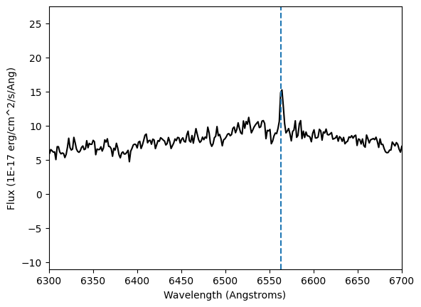
We just plotted our spectrum! Check different ranges of wavelength to see how the full spectrum looks like in comparison to the one we saw before.

Fit an Emission Line with a Gaussian Model

The blue dashed line marks the $H\alpha$ emission line. We can tell this is an active star because it has a strong emission line.

Now, we would like to measure the height of this line. Let's use astropy.modeling to fit a gaussian to the $H\alpha$ line. We are going to initialize a gaussian model at the position of the $H\alpha$ line. The idea is that the gaussian amplitude will tell us the height of the line.

gausian_model = models.Gaussian1D(1, 6563, 10)
fitter = fitting.LevMarLSQFitter()
gaussian_fit = fitter(gausian_model, lam, flux)

Let's plot the results.

plt.figure(figsize=(8,5))
plt.plot(lam, flux, color='k')
plt.plot(lam, gaussian_fit(lam), color='darkorange')
plt.xlim(6300,6700)
plt.xlabel('Wavelength (Angstroms)')
plt.ylabel('Flux ({})'.format(units_flux))
plt.show()

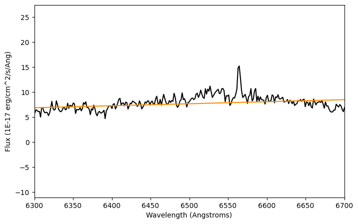
We can see the fit is not doing a good job. Let's print the parameters of this fit:

print(gaussian_fit)

Model: Gaussian1D
Inputs: ('x',)
Outputs: ('y',)
Model set size: 1
Parameters:
        amplitude             mean             stddev     
    ------------------ ----------------- -----------------
    16.750706286489784 9456.749529382625 2368.395705667002

Exercise

Go back to the previous plot and try to make the fit work. Note: Do not spend more than 10 minutes in this exercise. A couple of ideas to try:

• Is it not working because of the model we chose to fit? You can find more models to use here.
• Is it not working because of the fitter we chose?
• Is it not working because of the range of data we are fitting?
• Is it not working because how we are plotting the data?

Compound models

One model is not enough to make this fit work. We need to combine a couple of models to make a compound model in astropy. The idea is that we can add, divide or multiply models that already exist in astropy.modeling and fit the compound model to our data.

For our problem we are going to combine the gaussian with a polynomial of degree 1 to account for the background spectrum close to the $H\alpha$ line. Take a look at the plot we made before to convince yourself that this is the case.

Now let's make our compound model!

compound_model = models.Gaussian1D(1, 6563, 10) + models.Polynomial1D(degree=1)

After this point, we fit the data in exactly the same way as before, except we use a compound model instead of the gaussian model.

fitter = fitting.LevMarLSQFitter()
compound_fit = fitter(compound_model, lam, flux)

plt.figure(figsize=(8,5))
plt.plot(lam, flux, color='k')
plt.plot(lam, compound_fit(lam), color='darkorange')
plt.xlim(6300,6700)
plt.xlabel('Wavelength (Angstroms)')
plt.ylabel('Flux ({})'.format(units_flux))
plt.show()

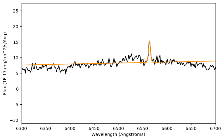
It works! Let's take a look to the fit we just made.

print(compound_fit)

Model: CompoundModel
Inputs: ('x',)
Outputs: ('y',)
Model set size: 1
Expression: [0] + [1]
Components: 
    [0]: <Gaussian1D(amplitude=7.02089174, mean=6564.13631715, stddev=1.97761475)>

    [1]: <Polynomial1D(1, c0=-12.79335619, c1=0.00323995)>
Parameters:
       amplitude_0          mean_0      ...         c0_1                c1_1        
    ----------------- ----------------- ... ------------------- --------------------
    7.020891743992038 6564.136317149307 ... -12.793356186323782 0.003239952053201798

Let's print all the parameters in a fancy way:

for x,y in zip(compound_fit.param_names, compound_fit.parameters):
    print(x,y)

amplitude_0 7.020891743992038
mean_0 6564.136317149307
stddev_0 1.9776147549595713
c0_1 -12.793356186323782
c1_1 0.003239952053201798

We can see that the result includes all the fit parameters from the gaussian (mean, std and amplitude) and the two coefficients from the polynomial of degree 1. So now if we want to see just the amplitude:

compound_fit.amplitude_0

Parameter('amplitude', value=7.020891743992038)

Conclusions: What was the difference between the first simple Gaussian and the compound model? The linear model that we added up to the gaussian model allowed the base of the Gaussian fit to have a slope and a background level. Normal Gaussians go to zero at $\pm \inf$; this one doesn't.

Fixed or bounded model parameters

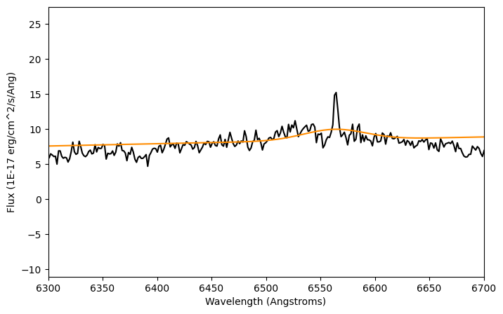
The mean value of the gaussian from our previous model indicates where the $H\alpha$ line is. In our fit result, we can tell that it is a little off from $6563$ Angstroms. One way to fix this is to fix some of the parameters of the model. In astropy.modeling these are called fixed parameters.

compound_model_fixed = models.Gaussian1D(1, 6563, 10) + models.Polynomial1D(degree=1)
compound_model_fixed.mean_0.fixed = True

Now let's use this new model with a fixed parameter to fit the data the same way we did before.

fitter = fitting.LevMarLSQFitter()
compound_fit_fixed = fitter(compound_model_fixed, lam, flux)

plt.figure(figsize=(8,5))
plt.plot(lam, flux, color='k')
plt.plot(lam, compound_fit_fixed(lam), color='darkorange')
plt.xlim(6300,6700)
plt.xlabel('Wavelength (Angstroms)')
plt.ylabel('Flux ({})'.format(units_flux))
plt.show()

print(compound_fit_fixed)

Model: CompoundModel
Inputs: ('x',)
Outputs: ('y',)
Model set size: 1
Expression: [0] + [1]
Components: 
    [0]: <Gaussian1D(amplitude=1.53257471, mean=6563., stddev=28.57847527)>

    [1]: <Polynomial1D(1, c0=-12.79103, c1=0.00323745)>
Parameters:
       amplitude_0     mean_0 ...        c0_1                c1_1        
    ------------------ ------ ... ------------------ --------------------
    1.5325747099672096 6563.0 ... -12.79103000338307 0.003237448628249798

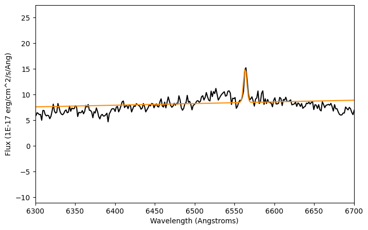
We can see in the plot that the height of the fit does not match the $H\alpha$ line height. What happend here is that we were too strict with the mean value, so we did not get a good fit. But the mean value is where we want it! Let's loosen this condition a little. Another thing we can do is to define a minimum and maximum value for the mean.

compound_model_bounded = models.Gaussian1D(1, 6563, 10) + models.Polynomial1D(degree=1)
delta = 0.5
compound_model_bounded.mean_0.max = 6563 + delta
compound_model_bounded.mean_0.min = 6563 - delta

fitter = fitting.LevMarLSQFitter()
compound_fit_bounded = fitter(compound_model_bounded, lam, flux)

plt.figure(figsize=(8,5))
plt.plot(lam, flux, color='k')
plt.plot(lam, compound_fit_bounded(lam), color='darkorange')
plt.xlim(6300,6700)
plt.xlabel('Wavelength (Angstroms)')
plt.ylabel('Flux ({})'.format(units_flux))
plt.show()

print(compound_fit_bounded)

Model: CompoundModel
Inputs: ('x',)
Outputs: ('y',)
Model set size: 1
Expression: [0] + [1]
Components: 
    [0]: <Gaussian1D(amplitude=6.65730507, mean=6563.5, stddev=2.09182676)>

    [1]: <Polynomial1D(1, c0=-12.79336254, c1=0.00323995)>
Parameters:
       amplitude_0    mean_0 ...         c0_1                 c1_1        
    ----------------- ------ ... ------------------- ---------------------
    6.657305067136674 6563.5 ... -12.793362542827573 0.0032399500254038354

Better! By loosening the condition we added to the mean value, we got a better fit and the mean of the gaussian is closer to where we want it.

Exercise

Modify the value of delta to change the minimum and maximum values for the mean of the gaussian. Look for:

• The better delta so the mean is closer to the real value of the $H\alpha$ line.
• What is the minimum delta for which the fit is still good according to the plot?

Custom model

What should you do if you need a model that astropy.modeling doesn't provide? To solve that problem, Astropy has another tool called custom model. Using this tool, we can create any model we want.

We will describe two ways to create a custom model:

• basic
• full

We use the basic custom model when we need a simple function to fit and the full custom model when we need a more complex function. Let's use an example to understand each one of the custom models.

Basic custom model

An Exponential Model is not provided by Astropy models. Let's see one example of basic custom model for this case. First, let's simulate a dataset that follows an exponential:

x1 = np.linspace(0,10,100)

a = 3
b = -2
c = 0
y1 = a*np.exp(b*x1+c)
y1 += np.random.normal(0., 0.2, x1.shape)
y1_err = np.ones(x1.shape)*0.2

plt.errorbar(x1 , y1, yerr=y1_err, fmt='.')
plt.show()

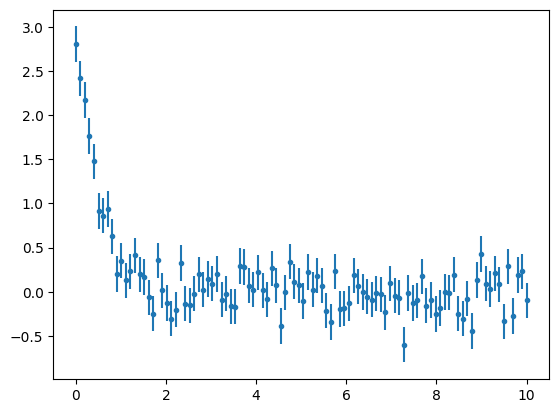
We can define a simple custom model by specifying which parameters we want to fit.

@custom_model
def exponential(x, a=1., b=1., c=1.):
    '''
    f(x)=a*exp(b*x + c)
    '''
    return a*np.exp(b*x+c)

Now we have one more available model to use in the same way we fit data with astropy.modeling.

exp_model = exponential(1.,-1.,1.)  
fitter = fitting.LevMarLSQFitter()
exp_fit = fitter(exp_model, x1, y1, weights = 1.0/y1_err**2)

plt.errorbar(x1 , y1, yerr=y1_err, fmt='.')
plt.plot(x1, exp_fit(x1))
plt.show()

print(exp_fit)

Model: exponential
Inputs: ('x',)
Outputs: ('y',)
Model set size: 1
Parameters:
            a                  b                  c         
    ------------------ ------------------ ------------------
    1.4900108822152918 -2.010051786355558 0.6934408519190175

The fit looks good in the plot. Let's check the parameters and the Reduced Chi Square value, which will give us information about the goodness of the fit.

def calc_reduced_chi_square(fit, x, y, yerr, N, n_free):
    '''
    fit (array) values for the fit
    x,y,yerr (arrays) data
    N total number of points
    n_free number of parameters we are fitting
    '''
    return 1.0/(N-n_free)*sum(((fit - y)/yerr)**2)

calc_reduced_chi_square(exp_fit(x1), x1, y1, y1_err, len(x1), 3)

np.float64(0.9751589771846978)

The Reduced Chi Square value is close to 1. Great! This means our fit is good, and we can corroborate it by comparing the values we got for the parameters and the ones we used to simulate the data.

Note: Fits of non-linear parameters (like in our example) are extremely dependent on initial conditions. Pay attention to the initial conditions you select.

Exercise

Modify the initial conditions of the fit and check yourself the relation between the best fit parameters and the initial conditions for the previous example. You can check it by looking at the Reduced Chi Square value: if it gets closer to 1 the fit is better and vice versa. To compare the quality of the fits you can take note of the Reduced Chi Square value you get for each initial condition.

Full custom model

What if we want to use a model from astropy.modeling, but with a different set of parameters? One example is the Sine Model. It has a very particular definition of the frequency and phase. Let's define a new Sine function with a full custom model. Again, first let's create a simulated dataset.

x2 = np.linspace(0,10,100)
a = 3
b = 2
c = 4
d = 1
y2 = a*np.sin(b*x2+c)+d
y2 += np.random.normal(0., 0.5, x2.shape)
y2_err = np.ones(x2.shape)*0.3

plt.errorbar(x2, y2, yerr=y2_err, fmt='.')
plt.show()

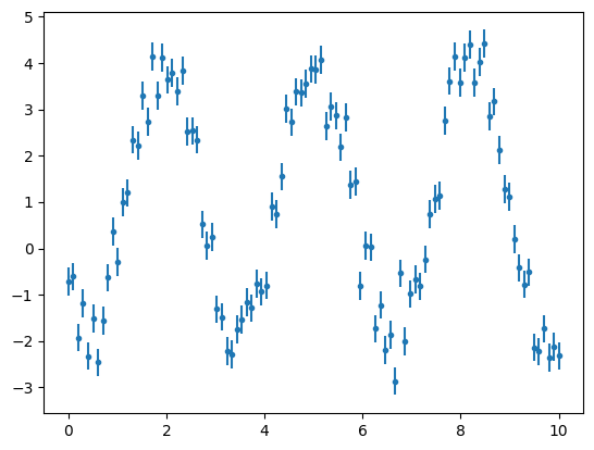
For the full custom model we can easily set the derivative of the function, which is used by different fitters, for example the LevMarLSQFitter().

class SineNew(Fittable1DModel):
    a = Parameter(default=1.)
    b = Parameter(default=1.)
    c = Parameter(default=1.)
    d = Parameter(default=1.)
        
    @staticmethod
    def evaluate(x, a, b, c, d):
        return a*np.sin(b*x+c)+d
    
    @staticmethod
    def fit_deriv(x, a, b, c, d):
        d_a = np.sin(b*x+c)
        d_b = a*np.cos(b*x+c)*x
        d_c = a*np.cos(b*x+c)
        d_d = np.ones(x.shape)
        return [d_a, d_b, d_c, d_d]

Note Defining default values for the fit parameters allows to define a model as model=SineNew()

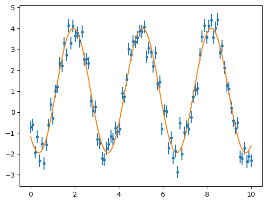
We are going to fit the data with our new model. Once more, the fit is very sensitive to the initial conditions due to the non-linearity of the parameters.

sine_model = SineNew(a=4.,b=2.,c=4.,d=0.)  
fitter = fitting.LevMarLSQFitter()
sine_fit = fitter(sine_model, x2, y2, weights = 1.0/y2_err**2)

plt.errorbar(x2, y2, yerr=y2_err, fmt='.')
plt.plot(x2,sine_fit(x2))
plt.show()

print(sine_fit)

Model: SineNew
Inputs: ('x',)
Outputs: ('y',)
Model set size: 1
Parameters:
            a                  b                  c                 d        
    ------------------ ------------------ ----------------- -----------------
    2.9906017626896815 2.0070002708298227 3.980508383219219 1.032960758023633

calc_reduced_chi_square(sine_fit(x2), x2, y2, y2_err, len(x2), 3)

np.float64(2.8233660558737363)

The Reduced Chi Squared value is showing the same as the plot: this fit could be improved. The Reduced Chi Squared is not close to 1 and the fit is off by small phase.

Exercise

Play with the initial values for the last fit and improve the Reduced Chi Squared value.

Note: A fancy way of doing this would be to code a function which iterates over different initial conditions, optimizing the Reduced Chi Squared value. No need to do it here, but feel free to try.

Exercise

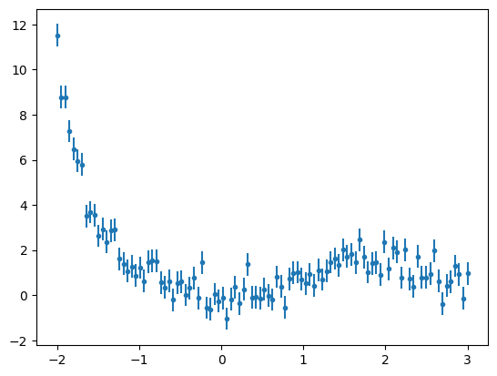
Custom models are also useful when we want to fit an unusual function to our data. As an example, create a full custom model to fit the following data.

x3 = np.linspace(-2,3,100)
y3 = x3**2* np.exp(-0.5 * (x3)**3 / 2**2)
y3 += np.random.normal(0., 0.5, x3.shape)
y3_err = np.ones(x3.shape)*0.5

plt.errorbar(x3,y3,yerr=y3_err,fmt='.')
plt.show()

Astropy footer