Learn.Astropy / Tutorials

Download

Outline

1. Authors
2. Learning Goals
3. Keywords
4. Summary
5. Index
6. Step 1: Download the data
7. Step 2: Load the cubes
8. Step 3: Convert cubes from frequency to velocity
   1. Create spatial maps of the peak intensity to quickly explore the cubes:

Cube Reprojection Tutorial

Authors

Adam Ginsburg, Eric Koch

Learning Goals

• reproject a cube spectrally
• smooth it spectrally
• reproject it spatially

Keywords

spectral cube, radio astronomy, astroquery, units, dask

Summary

Spectroscopic cube observations taken at different wavelength can trace the motion of gas or stars using spectral lines, but often lines at different wavelengths give different information. For example, one might observe a galaxy in the 21cm line of HI and the 115 GHz line of CO, or a protoplanetary disk in a line of N2H+ and a line of CO, or a galactic disk in the H-alpha and H-beta lines (in absorption or emission). In order to compare these data sets pixel-by-pixel, they must be placed onto a common grid with common resolution.

This tutorial shows how to take two spectral cubes observed toward the same part of the sky, but different frequencies, and put them onto the same grid using spectral-cube.

It uses astroquery to obtain line frequencies from splatalogue; this example uses radio-wavelength data for which Splatalogue's molecular line lists are appropriate. Finally, it shows how to do the reprojection using dask to enable parallelization.

with open('requirements.txt') as f:
    print(f"Required packages for this notebook:\n{f.read()}")

Required packages for this notebook:
astropy
dask
numpy
radio_beam
reproject
spectral_cube @ git+https://github.com/radio-astro-tools/spectral-cube  # as of: 2024-10-10 for issue with 'distutils'

Index

• Step 1: Download
• Step 2: Open files, collect metadata
• Step 3: Convert to velocity
• Step 4: Spectral Interpolation
• Step 5: Spatial Smoothing
• Step 6: Reprojection

In this example, we do spectral smoothing and interpolation (step 4) before spatial smoothing and interpolation (step 5), but if you have a varying-resolution cube (with a different beam size for each channel), you have to do spatial smoothing first. For more information see the spectral-cube documentation.

Step 1: Download the data

(you might not have to do this step, since you may already have data)

import numpy as np
from astropy.utils.data import download_file

We download two example spectral cubes of a point in the Galactic center from a permalink on the ALMA archives. These are moderately large files, with sizes 18 MB and 337 MB.

If you have trouble with these downloads, try changing to a different ALMA server (e.g., almascience.eso.org->almascience.nrao.edu) or increase the timeout. See the download_file documentation.

filename_1 = download_file("https://almascience.eso.org/dataPortal/member.uid___A001_X1465_X3a33.BrickMaser_sci.spw71.cube.I.manual.image.pbcor.fits",
                           cache=True)

filename_2 = download_file("https://almascience.eso.org/dataPortal/member.uid___A001_X87d_X141.a_sma1_sci.spw27.cube.I.pbcor.fits",
                          cache=True)

Step 2: Load the cubes

from spectral_cube import SpectralCube

/opt/hostedtoolcache/Python/3.12.7/x64/lib/python3.12/site-packages/tqdm/auto.py:21: TqdmWarning: IProgress not found. Please update jupyter and ipywidgets. See https://ipywidgets.readthedocs.io/en/stable/user_install.html
  from .autonotebook import tqdm as notebook_tqdm

cube1 = SpectralCube.read(filename_1)
cube1

WARNING: StokesWarning: Cube is a Stokes cube, returning spectral cube for I component [spectral_cube.io.core]

SpectralCube with shape=(75, 250, 250) and unit=Jy / beam:
 n_x:    250  type_x: RA---SIN  unit_x: deg    range:   266.534072 deg:  266.554577 deg
 n_y:    250  type_y: DEC--SIN  unit_y: deg    range:   -28.713958 deg:  -28.695975 deg
 n_s:     75  type_s: FREQ      unit_s: Hz     range: 139434992275.503 Hz:139503942362.300 Hz

cube2 = SpectralCube.read(filename_2)
cube2

WARNING: StokesWarning: Cube is a Stokes cube, returning spectral cube for I component [spectral_cube.io.core]

SpectralCube with shape=(478, 420, 420) and unit=Jy / beam:
 n_x:    420  type_x: RA---SIN  unit_x: deg    range:   266.537002 deg:  266.551600 deg
 n_y:    420  type_y: DEC--SIN  unit_y: deg    range:   -28.711371 deg:  -28.698569 deg
 n_s:    478  type_s: FREQ      unit_s: Hz     range: 216957714464.027 Hz:217190639088.700 Hz

The cubes are at different frequencies - 139 and 217 GHz.

The first cube covers the H2CS 4(1,3)-3(1,2) line at 139.483699 GHz.

The second covers SiO v=5-4 at 217.104984 GHz

We use the find_lines tool to query splatalogue with astroquery over the spectral range covered by the cube. It returns a table of matching lines. Note that some line names will be repeated because Splatalogue includes several different databases and most chemical species are present in all of these.

cube1.find_lines(chemical_name=' H2CS ').show_in_notebook()

WARNING: ExperimentalImplementationWarning: The line-finding routine is experimental.  Please report bugs on the Issues page: https://github.com/radio-astro-tools/spectral-cube/issues [spectral_cube.spectral_cube]

WARNING

: AstropyDeprecationWarning: show_in_notebook() is deprecated as of 6.1 and to create
         interactive tables it is recommended to use dedicated tools like:
         - https://github.com/bloomberg/ipydatagrid
         - https://docs.bokeh.org/en/latest/docs/user_guide/interaction/widgets.html#datatable
         - https://dash.plotly.com/datatable [warnings]

Table length=4

idx	species_id	name	chemical_name	resolved_QNs	linelist	LovasASTIntensity	lower_state_energy	upper_state_energy	sijmu2	sij	aij	intintensity	Lovas_NRAO	orderedfreq	lower_state_energy_K	upper_state_energy_K	orderedFreq	measFreq	upperStateDegen	moleculeTag	qnCode	labref_Lovas_NIST	rel_int_HFS_Lovas	unres_quantum_numbers	lineid	transition_in_space	transition_in_G358	obsref_Lovas_NIST	source_Lovas_NIST	telescope_Lovas_NIST	transitionBandColor	searchErrorMessage	sqlquery	requestnumber
0	210	H<sub>2</sub>CS	Thioformaldehyde	4( 1, 3)- 3( 1, 2)	JPL	0.17	16.1465	20.79917	30.51674	11.223	-4.44732		1	139483.41	23.23108	29.92519	<span style = 'color: #DC143C'></span>	139.48341 (0.28), <span style = 'color: #DC143C'>139.48341</span>	27	-46003	303			4 1 3 3 1 2	4065687	0	0	Lor84a	rho Oph B1	MMWO 4.9m	datatablegreen		None	0
1	210	H<sub>2</sub>CS	Thioformaldehyde	4( 1, 3)- 3( 1, 2)	CDMS		16.1329	20.78557	30.59661	11.251	-4.44619		0	139483.6816	23.21151	29.90563	<span style = 'color: #DC143C'></span>	139.4836816 (0.05), <span style = 'color: #DC143C'>139.4836816</span>	27	-46509	303			4 1 3 3 1 2	4066266	0	0				datatablegreen		None	0
2	210	H<sub>2</sub>CS	Thioformaldehyde	4( 1, 3)- 3( 1, 2)	SLAIM	0.17	16.133	20.78568	30.59472	3.75	-3.94426		0	139483.699	23.21165	29.90578	139.483699 (0.017), <span style = 'color: #DC143C'>139.483699</span>	139.483741 (0.024), <span style = 'color: #DC143C'>139.483741</span>	8.5	0	0	Mar05		4( 1, 3)- 3( 1, 2)	3744487	1	0				datatablegreen		None	0
3	210	H<sub>2</sub>CS	Thioformaldehyde	4(1,3)-3(1,2)	Lovas	0.17	0.0	0.0	0.0	0.0	0.0		0	139483.699	0.0	0.0	139.483699 (0.017), <span style = 'color: #DC143C'>139.483699</span>	<span style = 'color: #DC143C'></span>		0	0			4(1,3)-3(1,2)	3734199	0	0	Lor84a	rho Oph B1	MMWO 4.9m	datatablegreen		None	0

cube2.find_lines(chemical_name='SiO').show_in_notebook()

WARNING: ExperimentalImplementationWarning: The line-finding routine is experimental.  Please report bugs on the Issues page: https://github.com/radio-astro-tools/spectral-cube/issues [spectral_cube.spectral_cube]
WARNING: AstropyDeprecationWarning: show_in_notebook() is deprecated as of 6.1 and to create
         interactive tables it is recommended to use dedicated tools like:
         - https://github.com/bloomberg/ipydatagrid
         - https://docs.bokeh.org/en/latest/docs/user_guide/interaction/widgets.html#datatable
         - https://dash.plotly.com/datatable [warnings]

Table length=6

idx	species_id	name	chemical_name	resolved_QNs	linelist	LovasASTIntensity	lower_state_energy	upper_state_energy	sijmu2	sij	aij	intintensity	Lovas_NRAO	orderedfreq	lower_state_energy_K	upper_state_energy_K	orderedFreq	measFreq	upperStateDegen	moleculeTag	qnCode	labref_Lovas_NIST	rel_int_HFS_Lovas	unres_quantum_numbers	lineid	transition_in_space	transition_in_G358	obsref_Lovas_NIST	source_Lovas_NIST	telescope_Lovas_NIST	transitionBandColor	searchErrorMessage	sqlquery	requestnumber
0	21081	SiO, v = 0-10	Silicon monoxide (global fit)	J = 5 - 4, v = 0 - 0	CDMS		14.4843	21.72614	47.9909	0.0	-3.28429	-1.3211	1	217104.919	20.83981	31.25927	<span style = 'color: #DC143C'></span>	217.104919 (0.002), <span style = 'color: #DC143C'>217.104919</span>	11	-44505	1202			5 0 4 0	7980087	1	0	Belloche 2013	Sgr B2(N)	IRAM 30m	datatablelightpurple		None	0
1	20	SiO <font color="red">v = 0 </font>	Silicon Monoxide	5- 4	CDMS	1.6	14.4843	21.72614	47.99147	5.0	-3.28429		0	217104.98	20.83956	31.25889	<span style = 'color: #DC143C'></span>	217.10498 (0.08), <span style = 'color: #DC143C'>217.10498</span>	11	-44505	1202			5 0 4 0	6962437	0	0				datatablelightpurple		None	0
2	20	SiO <font color="red">v = 0 </font>	Silicon Monoxide	5- 4	CDMS	1.6	14.4843	21.72614	47.9911	5.0	-3.28429	-1.3199	0	217104.98	20.83956	31.25889	<span style = 'color: #DC143C'></span>	217.10498 (0.05), <span style = 'color: #DC143C'>217.10498</span>	11	-44505	1202			J=5-4 v=0	13358	1	0				datatablelightpurple		None	0
3	20	SiO <font color="red">v = 0 </font>	Silicon Monoxide	5-4	JPL	1.6	14.4843	21.72614	48.14651	5.0	-3.28288	-1.3166	1	217104.98	20.83956	31.25889	<span style = 'color: #DC143C'></span>	217.10498 (0.08), <span style = 'color: #DC143C'>217.10498</span>	11	-44002	101			J=5-4 v=0	1167368	0	0	Lor84a	OriMC-1	MMWO 4.9m	datatablelightpurple		None	0
4	20	SiO <font color="red">v = 0 </font>	Silicon Monoxide	5-4	Lovas	1.6	0.0	0.0	0.0	0.0	0.0		0	217104.984	0.0	0.0	217.104984 (0.014), <span style = 'color: #DC143C'>217.104984</span>	<span style = 'color: #DC143C'></span>		0	0			5-4 v=0	3724638	0	0	Lor84a	OriMC-1	MMWO 4.9m	datatablelightpurple		None	0
5	20	SiO <font color="red">v = 0 </font>	Silicon Monoxide	5 - 4	SLAIM		14.484	21.72584	47.6849	5.0	-3.28706		0	217104.984	20.83913	31.25846	217.104984 (0.014), <span style = 'color: #DC143C'>217.104984</span>	217.10498 (0.1), <span style = 'color: #DC143C'>217.10498</span>	11	0	0	Man77		5 - 4 v=0	3932866	0	0				datatablelightpurple		None	0

Step 3: Convert cubes from frequency to velocity

To compare the kinematic structure of the target, we need to convert from the observed frequency (which must be in a common reference frame; in this case, it already is) to the doppler velocity.

from astropy import units as u

cube1vel = cube1.with_spectral_unit(u.km/u.s, velocity_convention='radio', rest_value=139.483699*u.GHz)
cube1vel

SpectralCube with shape=(75, 250, 250) and unit=Jy / beam:
 n_x:    250  type_x: RA---SIN  unit_x: deg    range:   266.534072 deg:  266.554577 deg
 n_y:    250  type_y: DEC--SIN  unit_y: deg    range:   -28.713958 deg:  -28.695975 deg
 n_s:     75  type_s: VRAD      unit_s: km / s  range:      -43.509 km / s:     104.685 km / s

cube2vel = cube2.with_spectral_unit(u.km/u.s, velocity_convention='radio', rest_value=217.104984*u.GHz)
cube2vel

SpectralCube with shape=(478, 420, 420) and unit=Jy / beam:
 n_x:    420  type_x: RA---SIN  unit_x: deg    range:   266.537002 deg:  266.551600 deg
 n_y:    420  type_y: DEC--SIN  unit_y: deg    range:   -28.711371 deg:  -28.698569 deg
 n_s:    478  type_s: VRAD      unit_s: km / s  range:     -118.278 km / s:     203.359 km / s

From the shape of the cube, we can see the H2CS cube is narrower in velocity, so we'll use that as the target spectral reprojection. However, the SiO cube is the smaller footprint on the sky.

Create spatial maps of the peak intensity to quickly explore the cubes:

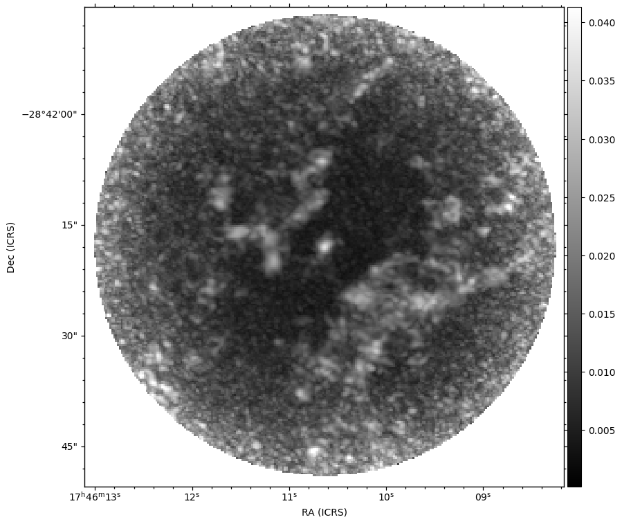
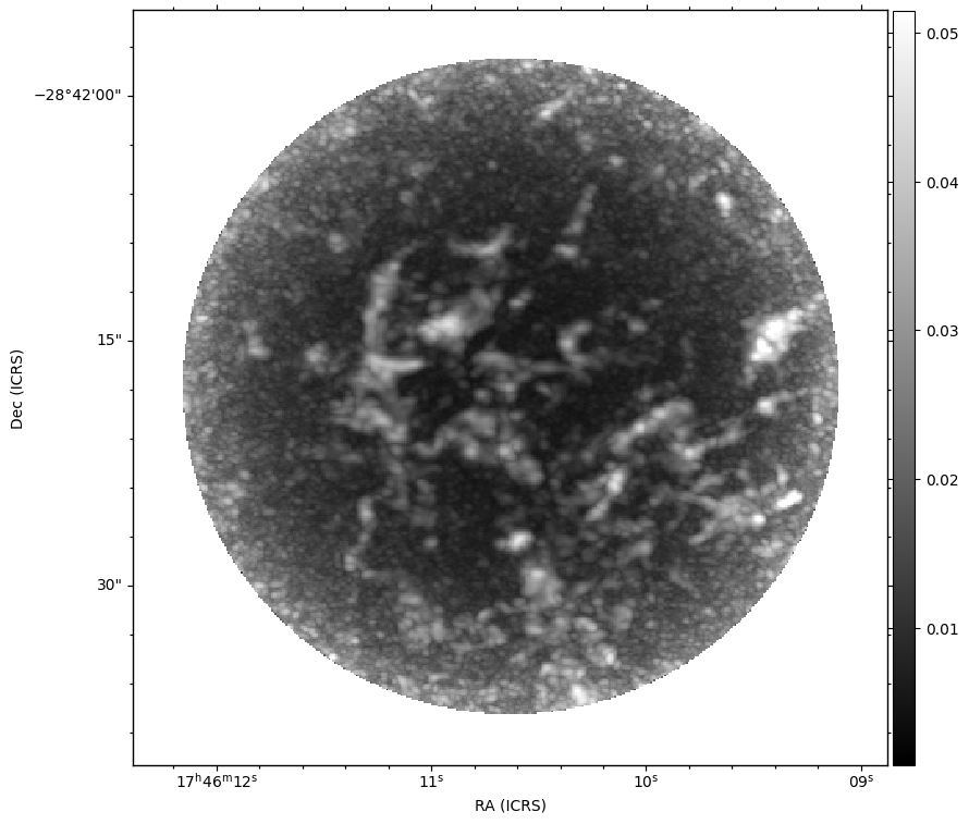
One way to quickly explore the structure in the data cubes is to produce a peak intensity map, or the maximum along the spectral axis (axis=0).

mx = cube1.max(axis=0)
mx.quicklook()

WARNING: PossiblySlowWarning: This function (<function BaseSpectralCube.max at 0x7ff760deb6a0>) requires loading the entire cube into memory and may therefore be slow. [spectral_cube.utils]
/opt/hostedtoolcache/Python/3.12.7/x64/lib/python3.12/site-packages/spectral_cube/spectral_cube.py:436: RuntimeWarning: All-NaN slice encountered
  out = function(self._get_filled_data(fill=fill,

We can do the same thing all on one line (for the other cube this time):

cube2.max(axis=0).quicklook()

WARNING: PossiblySlowWarning: This function (<function BaseSpectralCube.max at 0x7ff760deb6a0>) requires loading the entire cube into memory and may therefore be slow. [spectral_cube.utils]

/opt/hostedtoolcache/Python/3.12.7/x64/lib/python3.12/site-packages/spectral_cube/spectral_cube.py:436: RuntimeWarning: All-NaN slice encountered
  out = function(self._get_filled_data(fill=fill,

Step 4. Spectral Interpolation

We can choose to do either the spatial or spectral step first.
In this case, we choose the spectral step first because the H$_2$CS cube is narrower in velocity (cube1vel) and this will reduce the number of channels we need to spatially interpolate over in the next step.

We need to match resolution to the cube with the largest channel width:

velocity_res_1 = np.diff(cube1vel.spectral_axis)[0]
velocity_res_2 = np.diff(cube2vel.spectral_axis)[0]
velocity_res_1, velocity_res_2

(<Quantity 2.00262828 km / s>, <Quantity 0.67429189 km / s>)

Next, we will reduce cube2vel to have the same spectral range as cube1vel:

cube2vel_cutout = cube2vel.spectral_slab(cube1vel.spectral_axis.min(),
                                         cube1vel.spectral_axis.max())
cube1vel, cube2vel_cutout

(SpectralCube with shape=(75, 250, 250) and unit=Jy / beam:
  n_x:    250  type_x: RA---SIN  unit_x: deg    range:   266.534072 deg:  266.554577 deg
  n_y:    250  type_y: DEC--SIN  unit_y: deg    range:   -28.713958 deg:  -28.695975 deg
  n_s:     75  type_s: VRAD      unit_s: km / s  range:      -43.509 km / s:     104.685 km / s,
 SpectralCube with shape=(221, 420, 420) and unit=Jy / beam:
  n_x:    420  type_x: RA---SIN  unit_x: deg    range:   266.537002 deg:  266.551600 deg
  n_y:    420  type_y: DEC--SIN  unit_y: deg    range:   -28.711371 deg:  -28.698569 deg
  n_s:    221  type_s: VRAD      unit_s: km / s  range:      -43.432 km / s:     104.913 km / s)

Note that it is important for the to-be-interpolated cube, in this case cube2, to have pixels bounding cube1's spectral axis, but in this case it does not. If the pixel range doesn't overlap perfectly, it may blank out one of the edge pixels. So, to fix this, we add a little buffer:

cube2vel_cutout = cube2vel.spectral_slab(cube1vel.spectral_axis.min() - velocity_res_2,
                                         cube1vel.spectral_axis.max())
cube1vel, cube2vel_cutout

(SpectralCube with shape=(75, 250, 250) and unit=Jy / beam:
  n_x:    250  type_x: RA---SIN  unit_x: deg    range:   266.534072 deg:  266.554577 deg
  n_y:    250  type_y: DEC--SIN  unit_y: deg    range:   -28.713958 deg:  -28.695975 deg
  n_s:     75  type_s: VRAD      unit_s: km / s  range:      -43.509 km / s:     104.685 km / s,
 SpectralCube with shape=(222, 420, 420) and unit=Jy / beam:
  n_x:    420  type_x: RA---SIN  unit_x: deg    range:   266.537002 deg:  266.551600 deg
  n_y:    420  type_y: DEC--SIN  unit_y: deg    range:   -28.711371 deg:  -28.698569 deg
  n_s:    222  type_s: VRAD      unit_s: km / s  range:      -44.106 km / s:     104.913 km / s)

Our H2CS cube (cube1vel) has broader channels. We need to first smooth cube2vel to the broader channel width before doing the spatial reprojection.

To do this, we will spectrally smooth with a Gaussian with width set such that smoothing cube2vel will result in the same width as cube1vel. We do this by finding the difference in widths when deconvolving the cube1vel channel width from cube2vel. For further information see the documentation on smoothing.

Note that if we did not do this smoothing step, we would under-sample the cube2vel data in the next downsampling step, reducing our signal-to-noise ratio.

We have adopted a width equal to the channel width; the line spread function is actually a Hanning-smoothed tophat. We are making a coarse approximation here.

fwhm_gaussian = (velocity_res_1**2 - velocity_res_2**2)**0.5
fwhm_gaussian

$1.8856963 \; \mathrm{\frac{km}{s}}$

from astropy.convolution import Gaussian1DKernel
fwhm_to_sigma = np.sqrt(8*np.log(2))
# we want the kernel in pixel units, so we force to km/s and take the value
spectral_smoothing_kernel = Gaussian1DKernel(stddev=fwhm_gaussian.to(u.km/u.s).value / fwhm_to_sigma)

We then smooth with the kernel. Note that this is doing 420x420 = 176400 smoothing operations on a length-221 spectrum: it will take a little time

cube2vel_smooth = cube2vel_cutout.spectral_smooth(spectral_smoothing_kernel)

WARNING: nan_treatment='interpolate', however, NaN values detected post convolution. A contiguous region of NaN values, larger than the kernel size, are present in the input array. Increase the kernel size to avoid this. [astropy.convolution.convolve]

Now that we've done spectral smoothing, we can resample the spectral axis of cube2vel_smooth to match cube1vel by interpolating cube2vel_smooth onto cube1vel's grid:

cube2vel_spectralresample = cube2vel_smooth.spectral_interpolate(cube1vel.spectral_axis,
                                                                 suppress_smooth_warning=True)
cube2vel_spectralresample

Spectral Interpolate:   0%|          | 0/176400 [00:00<?, ?it/s]

Spectral Interpolate:   6%|▌         | 10691/176400 [00:00<00:01, 106906.79it/s]

Spectral Interpolate:  12%|█▏        | 21382/176400 [00:00<00:02, 60808.36it/s] 

Spectral Interpolate:  16%|█▌        | 28532/176400 [00:00<00:03, 40480.02it/s]

Spectral Interpolate:  19%|█▉        | 33576/176400 [00:00<00:04, 33984.75it/s]

Spectral Interpolate:  21%|██▏       | 37559/176400 [00:01<00:04, 30450.35it/s]

Spectral Interpolate:  23%|██▎       | 40922/176400 [00:01<00:04, 28481.41it/s]

Spectral Interpolate:  25%|██▍       | 43927/176400 [00:01<00:04, 26500.05it/s]

Spectral Interpolate:  26%|██▋       | 46643/176400 [00:01<00:05, 24792.43it/s]

Spectral Interpolate:  28%|██▊       | 49137/176400 [00:01<00:05, 23012.44it/s]

Spectral Interpolate:  29%|██▉       | 51427/176400 [00:01<00:05, 21923.18it/s]

Spectral Interpolate:  30%|███       | 53593/176400 [00:01<00:06, 19490.66it/s]

Spectral Interpolate:  31%|███▏      | 55551/176400 [00:01<00:06, 19511.28it/s]

Spectral Interpolate:  33%|███▎      | 57639/176400 [00:02<00:05, 19850.87it/s]

Spectral Interpolate:  34%|███▍      | 59628/176400 [00:02<00:06, 17387.08it/s]

Spectral Interpolate:  35%|███▍      | 61460/176400 [00:02<00:06, 17617.27it/s]

Spectral Interpolate:  36%|███▌      | 63254/176400 [00:02<00:07, 14658.47it/s]

Spectral Interpolate:  37%|███▋      | 64809/176400 [00:02<00:08, 13431.76it/s]

Spectral Interpolate:  38%|███▊      | 66744/176400 [00:02<00:07, 14810.74it/s]

Spectral Interpolate:  39%|███▉      | 68574/176400 [00:02<00:06, 15681.29it/s]

Spectral Interpolate:  40%|███▉      | 70452/176400 [00:02<00:06, 16494.59it/s]

Spectral Interpolate:  41%|████      | 72427/176400 [00:03<00:05, 17381.06it/s]

Spectral Interpolate:  42%|████▏     | 74220/176400 [00:03<00:06, 16864.32it/s]

Spectral Interpolate:  43%|████▎     | 76149/176400 [00:03<00:05, 17538.01it/s]

Spectral Interpolate:  44%|████▍     | 77958/176400 [00:03<00:05, 17693.79it/s]

Spectral Interpolate:  45%|████▌     | 79912/176400 [00:03<00:05, 18224.81it/s]

Spectral Interpolate:  46%|████▋     | 81784/176400 [00:03<00:05, 18367.00it/s]

Spectral Interpolate:  47%|████▋     | 83635/176400 [00:03<00:05, 17647.21it/s]

Spectral Interpolate:  48%|████▊     | 85415/176400 [00:03<00:05, 17665.19it/s]

Spectral Interpolate:  49%|████▉     | 87229/176400 [00:03<00:05, 17802.01it/s]

Spectral Interpolate:  51%|█████     | 89140/176400 [00:03<00:04, 18182.85it/s]

Spectral Interpolate:  52%|█████▏    | 90965/176400 [00:04<00:05, 15900.77it/s]

Spectral Interpolate:  53%|█████▎    | 92623/176400 [00:04<00:05, 16079.86it/s]

Spectral Interpolate:  54%|█████▎    | 94590/176400 [00:04<00:04, 17075.90it/s]

Spectral Interpolate:  55%|█████▍    | 96461/176400 [00:04<00:04, 17538.07it/s]

Spectral Interpolate:  56%|█████▌    | 98377/176400 [00:04<00:04, 18004.02it/s]

Spectral Interpolate:  57%|█████▋    | 100256/176400 [00:04<00:04, 18231.93it/s]

Spectral Interpolate:  58%|█████▊    | 102095/176400 [00:04<00:04, 18036.42it/s]

Spectral Interpolate:  59%|█████▉    | 104029/176400 [00:04<00:03, 18417.07it/s]

Spectral Interpolate:  60%|██████    | 106019/176400 [00:04<00:03, 18852.41it/s]

Spectral Interpolate:  61%|██████    | 107911/176400 [00:05<00:03, 17808.40it/s]

Spectral Interpolate:  62%|██████▏   | 109839/176400 [00:05<00:03, 18227.58it/s]

Spectral Interpolate:  63%|██████▎   | 111820/176400 [00:05<00:03, 18683.64it/s]

Spectral Interpolate:  64%|██████▍   | 113700/176400 [00:05<00:03, 17724.72it/s]

Spectral Interpolate:  65%|██████▌   | 115489/176400 [00:05<00:03, 17475.00it/s]

Spectral Interpolate:  67%|██████▋   | 117502/176400 [00:05<00:03, 18230.81it/s]

Spectral Interpolate:  68%|██████▊   | 119337/176400 [00:05<00:03, 16465.53it/s]

Spectral Interpolate:  69%|██████▊   | 121021/176400 [00:05<00:03, 16325.20it/s]

Spectral Interpolate:  70%|██████▉   | 122679/176400 [00:05<00:03, 15673.35it/s]

Spectral Interpolate:  71%|███████   | 124424/176400 [00:05<00:03, 16159.64it/s]

Spectral Interpolate:  72%|███████▏  | 126569/176400 [00:06<00:02, 17647.18it/s]

Spectral Interpolate:  73%|███████▎  | 128357/176400 [00:06<00:02, 16045.51it/s]

Spectral Interpolate:  74%|███████▎  | 130002/176400 [00:06<00:02, 15825.69it/s]

Spectral Interpolate:  75%|███████▍  | 132173/176400 [00:06<00:02, 17440.16it/s]

Spectral Interpolate:  76%|███████▋  | 134508/176400 [00:06<00:02, 19104.18it/s]

Spectral Interpolate:  77%|███████▋  | 136453/176400 [00:06<00:02, 18884.66it/s]

Spectral Interpolate:  78%|███████▊  | 138399/176400 [00:06<00:01, 19047.03it/s]

Spectral Interpolate:  80%|███████▉  | 140322/176400 [00:06<00:01, 18771.71it/s]

Spectral Interpolate:  81%|████████  | 142793/176400 [00:06<00:01, 20493.90it/s]

Spectral Interpolate:  82%|████████▏ | 145336/176400 [00:07<00:01, 21939.49it/s]

Spectral Interpolate:  84%|████████▍ | 148046/176400 [00:07<00:01, 23460.68it/s]

Spectral Interpolate:  86%|████████▌ | 150846/176400 [00:07<00:01, 24806.26it/s]

Spectral Interpolate:  87%|████████▋ | 153337/176400 [00:07<00:00, 23304.74it/s]

Spectral Interpolate:  88%|████████▊ | 155693/176400 [00:07<00:00, 21961.72it/s]

Spectral Interpolate:  90%|████████▉ | 158682/176400 [00:07<00:00, 24155.49it/s]

Spectral Interpolate:  92%|█████████▏| 162430/176400 [00:07<00:00, 27930.49it/s]

Spectral Interpolate:  97%|█████████▋| 170940/176400 [00:07<00:00, 44402.86it/s]

Spectral Interpolate: 100%|██████████| 176400/176400 [00:07<00:00, 22462.14it/s]

SpectralCube with shape=(75, 420, 420) and unit=Jy / beam:
 n_x:    420  type_x: RA---SIN  unit_x: deg    range:   266.537002 deg:  266.551600 deg
 n_y:    420  type_y: DEC--SIN  unit_y: deg    range:   -28.711371 deg:  -28.698569 deg
 n_s:     75  type_s: VRAD      unit_s: km / s  range:      -43.509 km / s:     104.685 km / s

Note that we included the suppress_smooth_warning=True argument. That is to hide this warning:

WARNING: SmoothingWarning: Input grid has too small a spacing. The data should be smoothed prior to resampling. [spectral_cube.spectral_cube]

which will tell you if the operation will under-sample the original data. The smoothing work we did above is specifically to make sure we are properly sampling, so this warning does not apply.

Step 5. Spatial Smoothing

Now that we've done spectral smoothing, we also need to follow a similar procedure of smoothing then resampling for the spatial axes.

The beam is the resolution element of our cubes:

cube1vel.beam, cube2vel_spectralresample.beam

(Beam: BMAJ=1.29719604986604 arcsec BMIN=1.04247149438736 arcsec BPA=82.95313553702 deg,
 Beam: BMAJ=0.8935712308515601 arcsec BMIN=0.6649610689789199 arcsec BPA=85.81119797802 deg)

cube1 again hase the larger beam, so we'll smooth cube2 to its resolution

Aside: mixed beams

If cube1 and cube2 had different sized beams, but neither was clearly larger, we would have to convolve both to a common beam.

In this case, it's redundant and we could have just used cube1's beam, but this is the more general approach:

import radio_beam
common_beam = radio_beam.commonbeam.common_2beams(radio_beam.Beams(beams=[cube1vel.beam, cube2vel.beam]))
common_beam

Beam: BMAJ=$1.29719604986604^{''}$ BMIN=$1.04247149438736^{''}$ BPA=$82.95313553702^\circ$

We then convolve:

# for v<0.6, we convert to Kelvin to ensure the units are preserved:
# cube2vel_spatialspectralsmooth = cube2vel_spectralresample.to(u.K).convolve_to(common_beam)
# in more recent versions, the unit conversion is handled appropriately,
# so unit conversion isn't needed
cube2vel_spatialspectralsmooth = cube2vel_spectralresample.convolve_to(common_beam)
cube2vel_spatialspectralsmooth

SpectralCube with shape=(75, 420, 420) and unit=Jy / beam:
 n_x:    420  type_x: RA---SIN  unit_x: deg    range:   266.537002 deg:  266.551600 deg
 n_y:    420  type_y: DEC--SIN  unit_y: deg    range:   -28.711371 deg:  -28.698569 deg
 n_s:     75  type_s: VRAD      unit_s: km / s  range:      -43.509 km / s:     104.685 km / s

Step 6. Reprojection

Now we can do the spatial resampling as the final step for producing two cubes matched to the same spatial and spectral pixel grid:

# first we make a copy of the target (cube1vel) header and set its rest frequency 
# to that of the cube we're reprojecting (cube2vel_spatialspectralsmooth)
# (see https://github.com/radio-astro-tools/spectral-cube/issues/874)
tgthdr = cube1vel.header
tgthdr['RESTFRQ'] = cube2vel_spatialspectralsmooth.header['RESTFRQ']

# now we continue with the reprojection
cube2vel_reproj = cube2vel_spatialspectralsmooth.reproject(tgthdr)
cube2vel_reproj

SpectralCube with shape=(75, 250, 250) and unit=Jy / beam:
 n_x:    250  type_x: RA---SIN  unit_x: deg    range:   266.534072 deg:  266.554577 deg
 n_y:    250  type_y: DEC--SIN  unit_y: deg    range:   -28.713958 deg:  -28.695975 deg
 n_s:     75  type_s: VRAD      unit_s: km / s  range:      -43.509 km / s:     104.685 km / s

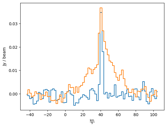
These two cubes are now on an identical grid, and can be directly compared:

cube2vel_reproj, cube1vel

(SpectralCube with shape=(75, 250, 250) and unit=Jy / beam:
  n_x:    250  type_x: RA---SIN  unit_x: deg    range:   266.534072 deg:  266.554577 deg
  n_y:    250  type_y: DEC--SIN  unit_y: deg    range:   -28.713958 deg:  -28.695975 deg
  n_s:     75  type_s: VRAD      unit_s: km / s  range:      -43.509 km / s:     104.685 km / s,
 SpectralCube with shape=(75, 250, 250) and unit=Jy / beam:
  n_x:    250  type_x: RA---SIN  unit_x: deg    range:   266.534072 deg:  266.554577 deg
  n_y:    250  type_y: DEC--SIN  unit_y: deg    range:   -28.713958 deg:  -28.695975 deg
  n_s:     75  type_s: VRAD      unit_s: km / s  range:      -43.509 km / s:     104.685 km / s)

These spectra can now be overplotted as they are in the same unit with the same beam.

cube1vel[:,125,125].quicklook()
cube2vel_reproj[:,125,125].quicklook()

Dask

All of the above can be done using dask as the underlying framework to parallelize the operations. See the spectral-cube documentation on dask integration or the dask documentation for further details.

The dask approach can be made more memory-efficient (avoid using too much RAM) by writing intermediate steps to disk. The non-dask approach used above will generally need to read the whole cube into memory. Depending on the situation, either approach may be faster, but dask may be needed if the cube is larger than memory.

We repeat all the operations above using dask. We use a ProgressBar so you can see how long it takes. We also suppress warnings to make the output look cleaner (we already saw all the important warnings above).

from dask.diagnostics import ProgressBar
import warnings

with warnings.catch_warnings():
    warnings.simplefilter('ignore')
    with ProgressBar():
        cube2dask = SpectralCube.read(filename_2, use_dask=True)
        cube2daskvel = cube2dask.with_spectral_unit(u.km/u.s,
                                            velocity_convention='radio', rest_value=217.104984*u.GHz)
        cube2daskvel_cutout = cube2daskvel.spectral_slab(cube1vel.spectral_axis.min() - velocity_res_2,
                                                 cube1vel.spectral_axis.max())
        cube2daskvel_smooth = cube2daskvel_cutout.spectral_smooth(spectral_smoothing_kernel)
        cube2daskvel_spectralresample = cube2daskvel_smooth.spectral_interpolate(cube1vel.spectral_axis,
                                                                             suppress_smooth_warning=True)
        cube2daskvel_spatialspectralsmooth = cube2daskvel_spectralresample.convolve_to(common_beam)
        cube2daskvel_reproj = cube2daskvel_spatialspectralsmooth.reproject(tgthdr) # as above, tgthdr is altered cube1vel header
cube2daskvel_reproj

[                                        ] | 0% Completed | 395.34 us

[                                        ] | 0% Completed | 101.61 ms

[                                        ] | 0% Completed | 205.18 ms

[                                        ] | 0% Completed | 452.08 ms

[                                        ] | 0% Completed | 700.30 ms

[                                        ] | 0% Completed | 824.72 ms

[                                        ] | 0% Completed | 1.60 s

[                                        ] | 0% Completed | 1.70 s

[                                        ] | 0% Completed | 1.92 s

[                                        ] | 0% Completed | 2.19 s

[                                        ] | 0% Completed | 2.29 s

[                                        ] | 0% Completed | 2.40 s

[                                        ] | 0% Completed | 3.23 s

[                                        ] | 0% Completed | 3.33 s

[                                        ] | 0% Completed | 3.44 s

[                                        ] | 0% Completed | 3.54 s

[                                        ] | 0% Completed | 152.72 s

[                                        ] | 0% Completed | 152.82 s

[                                        ] | 0% Completed | 152.93 s

[                                        ] | 0% Completed | 153.17 s

[                                        ] | 0% Completed | 153.39 s

[                                        ] | 0% Completed | 154.24 s

[                                        ] | 0% Completed | 154.34 s

[                                        ] | 0% Completed | 154.44 s

[########################################] | 100% Completed | 154.54 s

DaskSpectralCube with shape=(75, 250, 250) and unit=Jy / beam and chunk size (75, 250, 250):
 n_x:    250  type_x: RA---SIN  unit_x: deg    range:   266.534072 deg:  266.554577 deg
 n_y:    250  type_y: DEC--SIN  unit_y: deg    range:   -28.713958 deg:  -28.695975 deg
 n_s:     75  type_s: VRAD      unit_s: km / s  range:      -43.509 km / s:     104.685 km / s

Astropy footer