Viewing and manipulating data from FITS tables

Authors

Lia Corrales, Kris Stern

Learning Goals

• Download a FITS table file from a URL

• Open a FITS table file and view table contents

• Make a 2D histogram with the table data

• Close the FITS file after use

Keywords

FITS, file input/output, table, numpy, matplotlib, histogram

Summary

This tutorial demonstrates the use of astropy.utils.data to download a data file, then uses astropy.io.fits and astropy.table to open the file. Lastly, matplotlib is used to visualize the data as a histogram.

import numpy as np
from astropy.io import fits
from astropy.table import Table
from matplotlib.colors import LogNorm

# Set up matplotlib
import matplotlib.pyplot as plt

%matplotlib inline

The following line is needed to download the example FITS files used in this tutorial.

from astropy.utils.data import download_file

FITS files often contain large amounts of multi-dimensional data and tables.

In this particular example, we’ll open a FITS file from a Chandra observation of the Galactic Center. The file contains a list of events with x and y coordinates, energy, and various other pieces of information.

event_filename = download_file(
    "http://data.astropy.org/tutorials/FITS-tables/chandra_events.fits", cache=True
)

Opening the FITS file and viewing table contents

Since the file is big, let’s open it with memmap=True to prevent RAM storage issues.

hdu_list = fits.open(event_filename, memmap=True)

hdu_list.info()

Filename: /home/runner/.astropy/cache/download/url/333246bccb141ea3b4e86c49e45bf8d6/contents
No.    Name      Ver    Type      Cards   Dimensions   Format
  0  PRIMARY       1 PrimaryHDU      30   ()      
  1  EVENTS        1 BinTableHDU    890   483964R x 19C   [1D, 1I, 1I, 1J, 1I, 1I, 1I, 1I, 1E, 1E, 1E, 1E, 1J, 1J, 1E, 1J, 1I, 1I, 32X]   
  2  GTI           3 BinTableHDU     28   1R x 2C   [1D, 1D]   
  3  GTI           2 BinTableHDU     28   1R x 2C   [1D, 1D]   
  4  GTI           1 BinTableHDU     28   1R x 2C   [1D, 1D]   
  5  GTI           0 BinTableHDU     28   1R x 2C   [1D, 1D]   
  6  GTI           6 BinTableHDU     28   1R x 2C   [1D, 1D]   

In this case, we’re interested in reading EVENTS, which contains information about each X-ray photon that hit the detector.

To find out what information the table contains, let’s print the column names.

print(hdu_list[1].columns)

ColDefs(
    name = 'time'; format = '1D'; unit = 's'
    name = 'ccd_id'; format = '1I'
    name = 'node_id'; format = '1I'
    name = 'expno'; format = '1J'
    name = 'chipx'; format = '1I'; unit = 'pixel'; coord_type = 'CPCX'; coord_unit = 'mm'; coord_ref_point = 0.5; coord_ref_value = 0.0; coord_inc = 0.023987
    name = 'chipy'; format = '1I'; unit = 'pixel'; coord_type = 'CPCY'; coord_unit = 'mm'; coord_ref_point = 0.5; coord_ref_value = 0.0; coord_inc = 0.023987
    name = 'tdetx'; format = '1I'; unit = 'pixel'
    name = 'tdety'; format = '1I'; unit = 'pixel'
    name = 'detx'; format = '1E'; unit = 'pixel'; coord_type = 'LONG-TAN'; coord_unit = 'deg'; coord_ref_point = 4096.5; coord_ref_value = 0.0; coord_inc = 0.00013666666666667
    name = 'dety'; format = '1E'; unit = 'pixel'; coord_type = 'NPOL-TAN'; coord_unit = 'deg'; coord_ref_point = 4096.5; coord_ref_value = 0.0; coord_inc = 0.00013666666666667
    name = 'x'; format = '1E'; unit = 'pixel'; coord_type = 'RA---TAN'; coord_unit = 'deg'; coord_ref_point = 4096.5; coord_ref_value = 266.41519201128; coord_inc = -0.00013666666666667
    name = 'y'; format = '1E'; unit = 'pixel'; coord_type = 'DEC--TAN'; coord_unit = 'deg'; coord_ref_point = 4096.5; coord_ref_value = -29.012248288366; coord_inc = 0.00013666666666667
    name = 'pha'; format = '1J'; unit = 'adu'; null = 0
    name = 'pha_ro'; format = '1J'; unit = 'adu'; null = 0
    name = 'energy'; format = '1E'; unit = 'eV'
    name = 'pi'; format = '1J'; unit = 'chan'; null = 0
    name = 'fltgrade'; format = '1I'
    name = 'grade'; format = '1I'
    name = 'status'; format = '32X'
)

Now we’ll take this data and convert it into an astropy table. While it’s possible to access FITS tables directly from the .data attribute, using Table tends to make a variety of common tasks more convenient.

evt_data = Table(hdu_list[1].data)

For example, a preview of the table is easily viewed by simply running a cell with the table as the last line:

evt_data

Table length=483964

time	ccd_id	node_id	expno	chipx	chipy	tdetx	tdety	detx	dety	x	y	pha	pha_ro	energy	pi	fltgrade	grade	status
float64	int16	int16	int32	int16	int16	int16	int16	float32	float32	float32	float32	int32	int32	float32	int32	int16	int16	bool[32]
238623220.9093583	3	3	68	920	8	5124	3981	5095.641	4138.995	4168.0723	5087.772	3548	3534	13874.715	951	16	4	False .. False
238623220.9093583	3	1	68	437	237	4895	3498	4865.567	4621.1826	3662.1968	4915.9336	667	629	2621.1938	180	64	2	False .. False
238623220.9093583	3	2	68	719	289	4843	3780	4814.835	4340.254	3935.2207	4832.552	3033	2875	12119.018	831	8	3	False .. False
238623220.9093583	3	0	68	103	295	4837	3164	4807.3643	4954.385	3324.4644	4897.2754	831	773	3253.0364	223	0	0	False .. False
238623220.9093583	3	1	68	498	314	4818	3559	4788.987	4560.3276	3713.6343	4832.735	3612	3439	14214.382	974	64	2	False .. False
238623220.9093583	3	3	68	791	469	4663	3852	4635.4526	4268.053	3985.8496	4645.93	500	438	1952.7239	134	0	0	False .. False
238623220.9093583	3	3	68	894	839	4293	3955	4266.642	4165.3203	4044.5469	4267.605	835	713	3267.5334	224	0	0	False .. False
238623220.9093583	3	3	68	857	941	4191	3918	4164.815	4202.2256	3995.9353	4170.818	975	804	3817.0366	262	0	0	False .. False
238623220.9093583	3	3	68	910	959	4173	3971	4146.9937	4149.364	4046.3376	4146.9106	576	446	2252.7295	155	0	0	False .. False
...	...	...	...	...	...	...	...	...	...	...	...	...	...	...	...	...	...	...
238672393.54971933	1	3	15723	933	199	4933	5040	4902.907	3082.4956	5212.4995	4766.2295	1222	1181	4819.8286	331	0	0	False .. False
238672393.54971933	1	2	15723	596	412	4720	4703	4691.51	3418.9893	4853.5117	4595.8037	3142	3020	12536.866	859	10	6	False .. False
238672393.54971933	1	3	15723	1000	608	4524	5107	4494.713	3015.7185	5230.886	4353.018	658	585	2599.5652	179	0	0	False .. False
238672393.54971933	1	1	15723	270	917	4215	4377	4188.3325	3743.5957	4472.07	4134.221	3861	3463	15535.768	1024	16	4	False .. False
238672393.54971933	1	0	15723	232	988	4144	4339	4117.6147	3781.8774	4425.75	4068.4873	1680	1499	6653.0815	456	0	0	False .. False
238672393.59075934	0	1	15723	366	103	3164	4766	3140.9048	3356.3208	4733.6816	3048.5664	3621	3602	14362.482	984	0	0	False .. False
238672393.59075934	0	3	15723	937	646	3707	4195	3681.2122	3925.5452	4231.8354	3651.9724	3717	3486	14653.954	1004	8	3	False .. False
238672393.59075934	0	1	15723	406	687	3748	4726	3723.4014	3396.252	4762.421	3631.7224	1676	1536	6652.827	456	0	0	False .. False
238672393.59075934	0	1	15723	354	870	3931	4778	3906.07	3344.775	4834.99	3807.0835	2436	2165	9672.882	663	16	4	False .. False
238672393.63179934	6	1	15723	384	821	3259	2523	3230.9204	5596.8496	2519.2202	3401.0327	491	356	1875.9359	129	0	0	False .. False

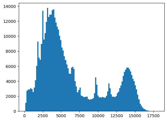
We can extract data from the table by referencing the column name. Let’s try making a histogram for the energy of each photon, which will give us a sense for the spectrum (folded with the detector’s efficiency).

energy_hist = plt.hist(evt_data["energy"], bins="auto")

Making a 2D histogram with some table data

We’ll make an image by binning the x and y coordinates of the events into a 2D histogram.

This particular observation spans five CCD chips. First, we determine the events that only fell on the main (ACIS-I) chips, which have number ids 0, 1, 2, and 3.

ii = np.in1d(evt_data["ccd_id"], [0, 1, 2, 3])
np.sum(ii)

/tmp/ipykernel_3551/3072746623.py:1: DeprecationWarning: `in1d` is deprecated. Use `np.isin` instead.
  ii = np.in1d(evt_data["ccd_id"], [0, 1, 2, 3])

np.int64(434858)

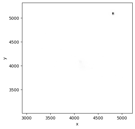
Method 1: Use numpy to make a 2D histogram and imshow to display it

This method allows us to create an image without stretching:

NBINS = (100, 100)

img_zero, yedges, xedges = np.histogram2d(evt_data["x"][ii], evt_data["y"][ii], NBINS)

extent = [xedges[0], xedges[-1], yedges[0], yedges[-1]]

plt.imshow(
    img_zero, extent=extent, interpolation="nearest", cmap="gist_yarg", origin="lower"
)

plt.xlabel("x")
plt.ylabel("y")

# To see more color maps
# http://wiki.scipy.org/Cookbook/Matplotlib/Show_colormaps

Text(0, 0.5, 'y')

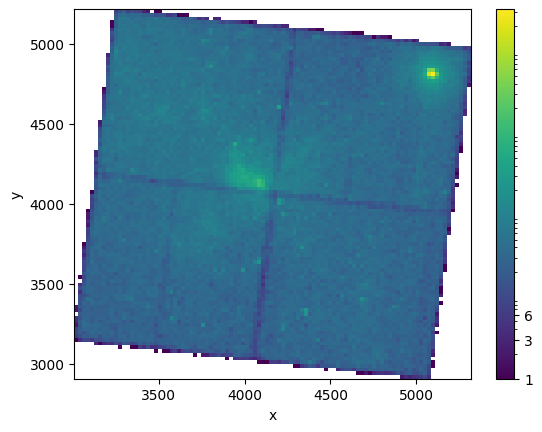
Method 2: Use hist2d with a log-normal color scheme

NBINS = (100, 100)
img_zero_mpl = plt.hist2d(
    evt_data["x"][ii], evt_data["y"][ii], NBINS, cmap="viridis", norm=LogNorm()
)

cbar = plt.colorbar(ticks=[1.0, 3.0, 6.0])
cbar.ax.set_yticklabels(["1", "3", "6"])

plt.xlabel("x")
plt.ylabel("y")

Text(0, 0.5, 'y')

Close the FITS file

When you’re done using a FITS file, it’s often a good idea to close it. That way you can be sure it won’t continue using up excess memory or file handles on your computer. (This happens automatically when you close Python, but you never know how long that might be…)

hdu_list.close()

Exercises

Make a scatter plot of the same data you histogrammed above. The plt.scatter function is your friend for this. What are the pros and cons of doing it this way?

Try the same with the plt.hexbin plotting function. Which do you think looks better for this kind of data?

Choose an energy range to make a slice of the FITS table, then plot it. How does the image change with different energy ranges?