Astronomical Coordinates 4: Cross-matching Catalogs Using astropy.coordinates and astroquery¶

Authors¶

Adrian Price-Whelan

Learning Goals¶

Demonstrate how to retrieve a catalog from Vizier using astroquery
Show how to perform positional cross-matches between catalogs of sky coordinates

Keywords¶

coordinates, OOP, astroquery, gaia

Summary¶

In the previous tutorials in this series, we introduced many of the key concepts underlying how to represent and transform astronomical coordinates using astropy.coordinates, including how to work with both position and velocity data within the coordinate objects.

In this tutorial, we will explore how the astropy.coordinates package can be used to cross-match two catalogs that contain overlapping sources that may have been observed at different times. You may find it helpful to keep the Astropy documentation for the coordinates package open alongside this tutorial for reference or additional reading. In the text below, you may also see some links that look like (docs). These links will take you to parts of the documentation that are directly relevant to the cells from which they link.

Note: This is the 4th tutorial in a series of tutorials about astropy.coordinates. If you are new to astropy.coordinates, you may want to start from the beginning or an earlier tutorial.

Previous tutorial: Astronomical Coordinates 3: Working with Velocity Data

In [1]:

with open('requirements.txt') as f:
    print(f"Required packages for this notebook:\n{f.read()}")

Required packages for this notebook:
astropy
astroquery>=0.4.8.dev9474  # 2024-09-24 pinned for Gaia column capitalization issue
matplotlib
numpy

Imports¶

We start by importing some general packages that we will need below:

In [2]:

import warnings

import matplotlib.pyplot as plt
%matplotlib inline
import numpy as np

from astropy import units as u
from astropy.coordinates import SkyCoord, Distance
from astropy.io import fits
from astropy.table import QTable
from astropy.time import Time
from astropy.utils.data import download_file

from astroquery.vizier import Vizier

Cross-matching and comparing catalogs¶

In this tutorial, we are going to return to a set of data that we downloaded from the Gaia archive back in Tutorial 1 of this series.

Let's recap what we did in that tutorial: We defined a SkyCoord object to represent the center of an open cluster (NGC 188), we queried the Gaia DR2 catalog to select stars that are close (on the sky) to the center of the cluster, and we used the parallax values from Gaia to select stars that are near NGC 188 in 3D position. Here, we will briefly reproduce those selections so that we can start here with a catalog of sources that are likely members of NGC 188 (see Tutorial 1 for more information):

In [3]:

ngc188_table = QTable.read('gaia_results.fits')
ngc188_table = ngc188_table[ngc188_table['parallax'] > 0.25*u.mas]

ngc188_center_3d = SkyCoord(12.11*u.deg, 85.26*u.deg,
                            distance=1.96*u.kpc,
                            pm_ra_cosdec=-2.3087*u.mas/u.yr,
                            pm_dec=-0.9565*u.mas/u.yr)

# Deal with masked quantity data in a backwards-compatible way:
parallax = ngc188_table['parallax']
if hasattr(parallax, 'mask'):
    parallax = parallax.filled(np.nan)
    
velocity_data = {
    'pm_ra_cosdec': ngc188_table['pmra'],
    'pm_dec': ngc188_table['pmdec'],
    'radial_velocity': ngc188_table['radial_velocity']
}
for k, v in velocity_data.items():
    if hasattr(v, 'mask'):
        velocity_data[k] = v.filled(0.)
    velocity_data[k][np.isnan(velocity_data[k])] = 0.

ngc188_coords_3d = SkyCoord(
    ra=ngc188_table['ra'], 
    dec=ngc188_table['dec'],
    distance=Distance(parallax=parallax),
    obstime=Time('J2015.5'),
    **velocity_data
)

sep3d = ngc188_coords_3d.separation_3d(ngc188_center_3d)
pm_diff = np.sqrt(
    (ngc188_table['pmra'] - ngc188_center_3d.pm_ra_cosdec)**2 + 
    (ngc188_table['pmdec'] - ngc188_center_3d.pm_dec)**2)

ngc188_members_mask = (sep3d < 50*u.pc) & (pm_diff < 1.5*u.mas/u.yr)
ngc188_members = ngc188_table[ngc188_members_mask]
ngc188_members_coords = ngc188_coords_3d[ngc188_members_mask]
len(ngc188_members)

Out[3]:

From the selections above, the table ngc188_members and the SkyCoord instance ngc188_members_coords contain 216 sources that, based on their 3D positions and proper motions, are consistent with being members of the open cluster NGC 188.

Let's assume that we now want to cross-match our catalog of candidate members of NGC 188 — here, based on Gaia data — to some other catalog. In this tutorial, we will demonstrate how to manually cross-match these Gaia sources with the 2MASS photometric catalog to retrieve infrared magnitudes for these stars, and then we will plot a color–magnitude diagram. To do this, we first need to query the 2MASS catalog to retrieve all sources in a region around the center of NGC 188, as we did for Gaia. Here, we will also take into account the fact that the Gaia data release 2 reference epoch is J2015.5, whereas the 2MASS coordinates are likely reported at their time of observation (in the late 1990's).

Note that some data archives, like the Gaia science archive, support running cross-matches at the database level and even support epoch propagation. If you need to perform a large cross-match, it will be much more efficient to use these services!

We will again use astroquery to execute this query. This will again require an internet connection, but we have included the results of this query in a file along with this notebook in case you are not connected to the internet. To query 2MASS, we will use the astroquery.vizier module (docs) to run a cone search centered on the sky position of NGC 188 with a search radius of 0.5º:

In [4]:

# NOTE: skip this cell if you do not have an internet connection

# II/246 is the catalog name for the main 2MASS photometric catalog
v = Vizier(catalog="II/246", columns=['*', 'Date'])  
v.ROW_LIMIT = -1

result = v.query_region(ngc188_center_3d, radius=0.5*u.deg)
tmass_table = result[0]

Alternatively, we can read the 2MASS table provided along with this tutorial:

In [5]:

# the .read() below produces some warnings that we can safely ignore
with warnings.catch_warnings(): 
    warnings.simplefilter('ignore', UserWarning)
    
    tmass_table = QTable.read('2MASS_results.ecsv')

As with the Gaia results table, we can now create a single SkyCoord object to represent all of the sources returned from our query to the 2MASS catalog. Let's look at the column names in this table by displaying the first few rows:

In [6]:

tmass_table[:3]

Out[6]:

QTable length=3

Date	RAJ2000	DEJ2000	_2MASS	Jmag	e_Jmag	Hmag	e_Hmag	Kmag	e_Kmag	Qflg	Rflg	Bflg	Cflg	Xflg	Aflg
	deg	deg		mag	mag	mag	mag	mag	mag
str10	float64	float64	str16	float32	float32	float32	float32	float32	float32	str3	str3	str3	str3	uint8	uint8
1999-10-19	9.633532	84.808350	00383204+8448300	13.079	0.030	12.742	0.033	12.729	0.035	AAA	222	111	000	0	0
1999-10-19	8.562472	84.873627	00341499+8452250	14.459	0.029	14.103	0.041	14.166	0.063	AAA	222	111	000	0	0
1999-10-19	8.645318	84.868584	00343487+8452069	10.356	0.026	10.057	0.032	10.000	0.020	AAA	222	111	000	0	0

From looking at the column names, the two relevant sky coordinate columns are RAJ2000 for ra and DEJ2000 for dec:

In [7]:

tmass_coords = SkyCoord(tmass_table['RAJ2000'], 
                        tmass_table['DEJ2000'])
len(tmass_coords)

Out[7]:

Note also that the table contains a "Date" column that specifies the epoch of the coordinates. Are all of these epochs the same?

In [8]:

np.unique(tmass_table['Date'])

Out[8]:

1999-10-19

It looks like all of the sources in our 2MASS table have the same epoch, so let's create an astropy.time.Time object to represent this date:

In [9]:

tmass_epoch = Time(np.unique(tmass_table['Date']))

We now want to cross-match our Gaia-selected candidate members of NGC 188, ngc_members_coords, with this table of photometry from 2MASS. However, as noted previously, the Gaia coordinates are given at a different epoch J2015.5, which is nearly ~16 years after the 2MASS epoch of the data we downloaded (1999-10-19 or roughly J1999.88). We will therefore first use the SkyCoord.apply_space_motion() method (docs) to transform the Gaia positions back to the 2MASS epoch before we do the cross-match:

In [10]:

# you can ignore the warning raised here
ngc188_members_coords_1999 = ngc188_members_coords.apply_space_motion(
    tmass_epoch)

The object ngc188_members_coords_1999 now contains the coordinate information for our Gaia-selected members of NGC 188, as we think they would appear if observed on 1999-10-19.

We can now use the SkyCoord.match_to_catalog_sky method to match these two catalogs (docs), using the ngc188_members_coords_1999 as our NGC 188 members coordinates.

Note that order matters with this method: Here we will match Gaia to 2MASS. SkyCoord.match_to_catalog_sky returns three objects: (1) the indices into tmass_coords that get the closest matches in ngc188_members_coords_1999, (2) the angular separation between each ngc188_members_coords_1999 coordinate and the closest source in tmass_coords, and (3) the 3D distance between each ngc188_members_coords_1999 coordinate and the closest source in tmass_coords. Here, the 3D distances will not be useful because the 2MASS coordinates do not have associated distance information, so we will ignore these quantities:

In [11]:

idx_gaia, sep2d_gaia, _ = ngc188_members_coords_1999.match_to_catalog_sky(
    tmass_coords)

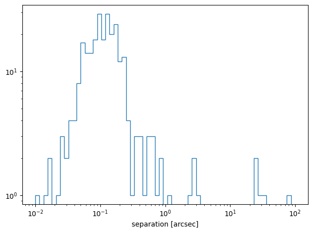
Let's now look at the distribution of separations (in arcseconds) for all of the cross-matched sources:

In [12]:

plt.hist(sep2d_gaia.arcsec, histtype='step', 
         bins=np.logspace(-2, 2., 64))
plt.xlabel('separation [arcsec]')
plt.xscale('log')
plt.yscale('log')
plt.tight_layout()

No description has been provided for this image

From this, it looks like all of sources in our Gaia NGC 188 member list cross-match to another sources within a few arcseconds, so these all seem like they are correctly matches to a 2MASS source!

In [13]:

(sep2d_gaia < 2*u.arcsec).sum(), len(ngc188_members)

Out[13]:

(np.int64(256), 265)

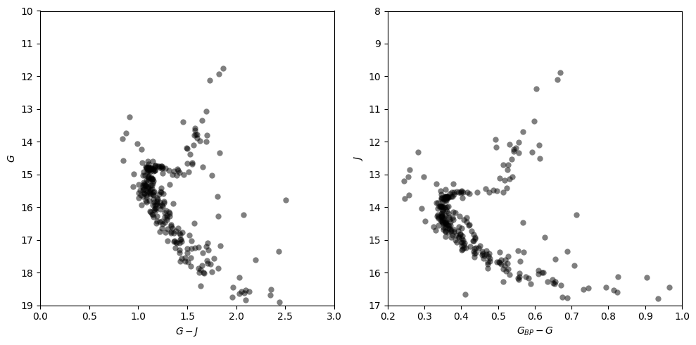
With our cross-match done, we can now make Gaia+2MASS color–magnitude diagrams of our candidate NGC 188 members using the information returned by the cross-match:

In [14]:

Jmag = tmass_table['Jmag'][idx_gaia]  # note that we use the index array returned above
Gmag = ngc188_members['phot_g_mean_mag']
Bmag = ngc188_members['phot_bp_mean_mag']

In [15]:

fig, axes = plt.subplots(1, 2, figsize=(10, 5))

ax = axes[0]
ax.scatter(Gmag - Jmag, Gmag, 
           marker='o', color='k', 
           linewidth=0, alpha=0.5)
ax.set_xlabel('$G - J$')
ax.set_ylabel('$G$')
ax.set_xlim(0, 3)
ax.set_ylim(19, 10) # backwards because magnitudes!

ax = axes[1]
ax.scatter(Bmag - Gmag, Jmag, 
           marker='o', color='k', 
           linewidth=0, alpha=0.5)
ax.set_xlabel('$G_{BP} - G$')
ax.set_ylabel('$J$')
ax.set_xlim(0.2, 1)
ax.set_ylim(17, 8) # backwards because magnitudes!

fig.tight_layout()

Those both look like color-magnitude diagrams of a main sequence + red giant branch of an intermediate-age stellar cluster, so it looks like our selection and cross-matching has worked!

For more on what matching options are available, check out the separation and matching section of the Astropy documentation. Or for more on what you can do with SkyCoord, see its API documentation.

In [ ]: