Astronomical Coordinates 2: Transforming Coordinate Systems and Representations#
Learning Goals#
Introduce key concepts in
astropy.coordinates: coordinate component formats, representations, and framesDemonstrate how to work with coordinate representations, for example, to change from Cartesian to Cylindrical coordinates
Introduce coordinate frame transformations and demonstrate transforming from ICRS coordinates to Galactic and Altitude-Azimuth coordinates
Keywords#
coordinates, OOP
Summary#
In the previous tutorial in this series, we showed how astronomical coordinates in the ICRS or equatorial coordinate system can be represented in Python using the SkyCoord object (docs). There are many other coordinate systems that are commonly used in astronomical research. For example, the Galactic coordinate system is often used in radio astronomy and Galactic science, the “horizontal” or altitude-azimuth frame is often used for observatory-specific observation planning, and Ecliptic coordinates are often used for solar system science or space mission footprints. All of these coordinate frames (and others!) are supported by astropy.coordinates. As we will see below, the SkyCoord object is designed to make transforming between these systems a straightforward task.
In this tutorial, we will explore how the astropy.coordinates package can be used to transform astronomical coordinates between different coordinate systems or frames. You may find it helpful to keep the Astropy documentation for the coordinates package open alongside this tutorial for reference or additional reading. In the text below, you may also see some links that look like (docs). These links will take you to parts of the documentation that are directly relevant to the cells from which they link.
Note: This is the 2nd tutorial in a series of tutorials about astropy.coordinates. If you are new to astropy.coordinates, you may want to start from the beginning or an earlier tutorial.
Imports#
We start by importing some general packages that we will need below:
import matplotlib as mpl
import matplotlib.pyplot as plt

%matplotlib inline
import numpy as np

from astropy import units as u
from astropy.coordinates import SkyCoord, Galactic, EarthLocation, AltAz
import astropy.coordinates as coord
from astropy.table import QTable
from astropy.time import Time
Key astropy.coordinates Concepts: Component Formats, Representations, and Frames#
Usage of the term “coordinates” is overloaded in astronomy and is often used interchangeably when referring to data formats (e.g., sexagesimal vs. decimal), representations (e.g., Cartesian vs. spherical), and frames (e.g., equatorial vs. galactic). In astropy.coordinates, we have tried to formalize these three concepts and have made them a core part of the way we interact with objects in this subpackage (docs). Here we will give an overview of these different concepts as we build up to demonstrating how to transform between different astronomical reference frames or systems.
Coordinate Component Formats#
In our previous tutorial, we showed that it is possible to pass in coordinate component data to the SkyCoord initializer as strings or as Quantity objects in a variety of formats and units. We also saw that the coordinate components of SkyCoord objects can be re-formatted. For example, we can change the coordinate format by changing the component units, or converting the data to a string:
c = SkyCoord(ra=15.9932 * u.deg, dec=-10.52351344 * u.deg)
print(c.ra.hourangle)
print(c.to_string("hmsdms"))
print(c.dec.to_string(sep=":", precision=5))
1.0662133333333335
01h03m58.368s -10d31m24.648384s
-10:31:24.64838
See the previous tutorial Astronomical Coordinates 1 - Getting Started for more examples of this.
Coordinate Representations#
In the previous tutorial, we only worked with coordinate data in spherical representations (longitude/latitude), but astropy.coordinates also supports other coordinate representations like Cartesian, cylindrical, etc. (docs). To retrieve the coordinate data in a different representation, we can use the SkyCoord.represent_as() method. This method either takes a string name of the desired representation, for example:
c.represent_as("cartesian")
<CartesianRepresentation (x, y, z) [dimensionless]
    (0.94512547, 0.27088898, -0.18263903)>
or it accepts an astropy.coordinates Representation class, such as:
c.represent_as(coord.CartesianRepresentation)
<CartesianRepresentation (x, y, z) [dimensionless]
    (0.94512547, 0.27088898, -0.18263903)>
A list of all supported representations is given in the documentation (docs), or can be identified as class names that end in Representaton:
print(
    [x for x in dir(coord) if x.endswith("Representation") and not x.startswith("Base")]
)
['CartesianRepresentation', 'CylindricalRepresentation', 'GRS80GeodeticRepresentation', 'PhysicsSphericalRepresentation', 'RadialRepresentation', 'SphericalRepresentation', 'UnitSphericalRepresentation', 'WGS72GeodeticRepresentation', 'WGS84GeodeticRepresentation']
In the SkyCoord object that we defined above, we only specified sky positions (i.e., no distance data), so the units of the Cartesian components that are returned above are dimensionless and are interpreted as being on the surface of the (dimensionless) unit sphere. If we instead pass in a distance to SkyCoord using the distance keyword argument, we instead get a CartesianRepresentation object for the 3D position with positional units. For example:
c2 = SkyCoord(ra=15.9932 * u.deg, dec=-10.52351344 * u.deg, distance=127.4 * u.pc)
c2.represent_as("cartesian")
<CartesianRepresentation (x, y, z) in pc
    (120.40898448, 34.5112558, -23.2682118)>
Or, we could represent this data with cylindrical components:
c2.represent_as("cylindrical")
<CylindricalRepresentation (rho, phi, z) in (pc, rad, pc)
    (125.2571368, 0.279134, -23.2682118)>
To summarize, using SkyCoord.represent_as() is a convenient way to retrieve your coordinate data in a different representation, like Cartesian or Cylindrical. You can also change (in place) the representation of a SkyCoord object by setting the SkyCoord.representation_type attribute. For example, if we create a SkyCoord again with a distance, the default representation type is spherical:
c3 = SkyCoord(ra=15.9932 * u.deg, dec=-10.52351344 * u.deg, distance=127.4 * u.pc)
print(c3.representation_type)
c3
<class 'astropy.coordinates.representation.spherical.SphericalRepresentation'>
<SkyCoord (ICRS): (ra, dec, distance) in (deg, deg, pc)
    (15.9932, -10.52351344, 127.4)>
We can, however, change the internal representation of the data by setting the representation_type attribute to a new Representation class:
c3.representation_type = coord.CylindricalRepresentation
This then changes the way SkyCoord will display the components:
c3
<SkyCoord (ICRS): (rho, phi, z) in (pc, deg, pc)
    (125.2571368, 15.9932, -23.2682118)>
Note, however, that changing the representation will also change the components that are available on a given SkyCoord object: Once we set the representation_type to cylindrical, the attributes .ra and .dec will no longer work, and we instead have to use the cylindrical component names to access the data. In this case, these are .rho for radius, .phi for azimuth, .z for \(z\) position:
c3.rho, c3.phi, c3.z
(<Quantity 125.2571368 pc>, <Angle 15.9932 deg>, <Quantity -23.2682118 pc>)
Transforming Between Coordinate Frames#
The third key concept to keep in mind when thinking about astronomical coordinate data is the reference frame or coordinate system that the data are in. In the previous tutorial, and so far here, we have worked with the default frame assumed by SkyCoord: the International Celestial Reference System (ICRS; some important definitions and context about the ICRS is given here). The ICRS is the fundamental coordinate system used in most modern astronomical contexts and is generally what people mean when they refer to “equatorial” or “J2000” or “RA/Dec” coordinates (but there are some important caveats if you are working with older data). As noted above, however, there are many other coordinate systems used in different astronomical, solar, or solar system contexts.
Some other common coordinate systems are defined as a rotation away from the ICRS that is defined to make science applications easier to interpret. One example here is the Galactic coordinate system, which is rotated with respect to the ICRS to approximately align the Galactic plane with latitude=0. As an example of the astropy.coordinates frame transformation machinery, we will load in a subset of a catalog of positions and distances to a set of open clusters in the Milky Way from Cantat-Gaudin et al. 2018 (Table 1 in this catalog). We have pre-selected the 474 clusters within 2 kpc of the sun and provide the catalog as a data file next to this notebook. This catalog provides sky position (columns RAJ2000 and DEJ2000 in the original catalog) and distance estimates (column dmode in the original catalog), which we have renamed in the table we provide to column names 'ra', 'dec', and 'distance'. We will start by loading the catalog as a QTable using astropy.table (docs):
tbl = QTable.read("Cantat-Gaudin-open-clusters.ecsv")
We can now pass the coordinate components to SkyCoord to create a single array-valued SkyCoord object to represent the positions of all of the open clusters in this catalog. Note that below we will explicitly specify the coordinate frame using frame='icrs': Even though this is the default frame, it is often better to be explicit so that it is clearer to someone reading the code what the coordinate system is:
open_cluster_c = SkyCoord(
    ra=tbl["ra"], dec=tbl["dec"], distance=tbl["distance"], frame="icrs"
)
len(open_cluster_c)
474
To see the first few coordinate entries, we can “slice” the array-valued coordinate object like we would a Python list or numpy array:
open_cluster_c[:4]
<SkyCoord (ICRS): (ra, dec, distance) in (deg, deg, pc)
    [( 51.87 , 34.981,  629.6), (288.399, 36.369,  382.2),
     (295.548, 27.366,  522.9), (298.306, 39.349, 1034.6)]>
Let’s now visualize the sky positions of all of these clusters, colored by their distances. To plot these in an all-sky spherical projection (e.g., aitoff) using matplotlib, with longitude increasing to the left as is typically done for plotting astronomical objects on the sky, we have to trick matplotlib a little bit: We have to pass in the negative angle values when plotting, then reformat the tick labels to make them positive values again. We have written a short function below to handle this trick:
def coordinates_aitoff_plot(coords):
    fig, ax = plt.subplots(figsize=(10, 4), subplot_kw=dict(projection="aitoff"))

    sph = coords.spherical
    cs = ax.scatter(
        -sph.lon.wrap_at(180 * u.deg).radian, sph.lat.radian, c=sph.distance.value
    )

    def fmt_func(x, pos):
        val = coord.Angle(-x * u.radian).wrap_at(360 * u.deg).degree
        return f"${val:.0f}" + r"^{\circ}$"

    ticker = mpl.ticker.FuncFormatter(fmt_func)
    ax.xaxis.set_major_formatter(ticker)

    ax.grid()

    cb = fig.colorbar(cs)
    cb.set_label("distance [pc]")

    return fig, ax
Now we can plot the sky positions by passing our SkyCoord object in to this coordinates_aitoff_plot() plot helper function:
fig, ax = coordinates_aitoff_plot(open_cluster_c)
ax.set_xlabel("RA [deg]")
ax.set_ylabel("Dec [deg]")
Text(0, 0.5, 'Dec [deg]')
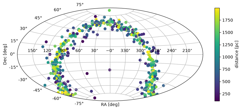
The majority of these open clusters are relatively close to the Galactic midplane, which is why they form a fairly narrow “band” on the sky in ICRS coordinates. If we transform these positions to Galactic coordinates, we would therefore expect the points to appear around the latitude \(b=0\) line.
To transform our coordinates from ICRS to Galactic (or any other coordinate system), we can use the SkyCoord.transform_to() method and pass in the new coordinate frame instance (in this case, Galactic()):
open_cluster_gal = open_cluster_c.transform_to(Galactic())
While the recommended way of transforming SkyCoord objects to new frames is by passing in a frame class instance as we demonstrated in the cell above, SkyCoord also supports a shorthand for transforming some frames by accessing attributes (named as the lower-case version of the new frame name):
open_cluster_gal = open_cluster_c.galactic
The transformed SkyCoord object now contains coordinate data in the Galactic coordinate frame:
open_cluster_gal[:4]
<SkyCoord (Galactic): (l, b, distance) in (deg, deg, pc)
    [(155.72353157, -17.76999215,  629.59997559),
     ( 68.02807936,  11.60790067,  382.20001221),
     ( 62.82445527,   2.06275608,  522.90002441),
     ( 74.37841053,   6.07393592, 1034.59997559)]>
Comparing this to the original SkyCoord, note that the names of the longitude and latitude components have changed from ra to l and from dec to b, per convention. We can therefore access the new Galactic longitude/latitude data using these new attribute names:
open_cluster_gal.l[:3]
open_cluster_gal.b[:3]
Note: the ICRS coordinate component names (.ra, .dec) will therefore not work on this new, transformed SkyCoord instance, open_cluster_gal
With this new SkyCoord object (in the Galactic frame), let’s re-make a sky plot to visualize the sky positions of the open clusters in Galactic coordinates:
fig, ax = coordinates_aitoff_plot(open_cluster_gal)
ax.set_xlabel("Galactic longitude, $l$ [deg]")
ax.set_ylabel("Galactic latitude, $b$ [deg]")
Text(0, 0.5, 'Galactic latitude, $b$ [deg]')
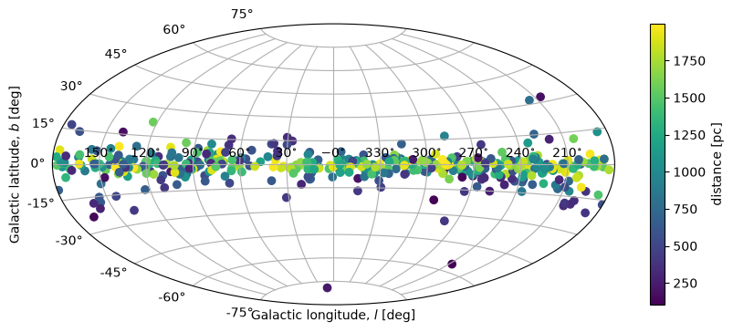
As we hoped and expected, in the Galactic coordinate frame, the open clusters predominantly appear at low galactic latitudes!
Transforming to More Complex Coordinate Frames: Computing the Altitude of a Target at an Observatory#
To determine whether a target is observable from a given observatory on Earth or to find out what targets are observable from a city or place on Earth at some time, we sometimes need to convert a coordinate or set of coordinates to a frame that is local to an on-earth observer. The most common choice for such a frame is “horizontal” or “Altitude-Azimuth” coordinates. In this frame, the sky coordinates of a source can be specified as an altitude from the horizon and an azimuth angle at a specified time. This coordinate frame is supported in astropy.coordinates through the AltAz coordinate frame.
The AltAz frame is different from the previously-demonstrated Galactic frame in that it requires additional metadata to define the frame instance. Since the Galactic frame is close to being a 3D rotation away from the ICRS frame, and that rotation matrix is fixed, we could transform to Galactic by instantiating the class with no arguments (see the example above where we used .transform_to(Galactic())). In order to specify an instance of the AltAz frame, we have to (at minimum) pass in (1) a location on Earth, and (2) the time (or times) we are requesting the frame at.
In astropy.coordinates, we specify locations on Earth with the EarthLocation class (docs). If we know the Earth longitude and latitude of our site, we can use these to create an instance of EarthLocation directly:
demo_loc = EarthLocation.from_geodetic(lon=-74.32834 * u.deg, lat=43.05885 * u.deg)
The EarthLocation class also provides handy short-hands for retrieving an instance for a given street address (by querying the OpenStreetMap web API):
demo_loc = EarthLocation.of_address("162 Fifth Ave, New York, NY 10010")
Or for an astronomical observatory (use EarthLocation.get_site_names() to see a list of all available sites). For example, to retrieve an EarthLocation instance for the position of Kitt Peak National Observatory (in AZ, USA):
observing_location = EarthLocation.of_site("Kitt Peak")
We will use Kitt Peak as our site.
As an example, we will now compute the altitude of a few of the open clusters from our catalog above over the course of a night. We have an object to represent our location on Earth, so now we need to create a set of times to compute the AltAz frame for. AltAz expects time information to be passed in as an astropy.time.Time object (docs; which can contain an array of times). Let’s pretend we have an observing run coming up on Dec 18, 2020, and we would like to compute the altitude/azimuth coordinates for our open clusters over that whole night.
# 1AM UTC = 6PM local time (AZ mountain time), roughly the start of a night
observing_date = Time("2020-12-18 1:00")

# Compute the alt/az over a 14 hour period, starting at 6PM local time,
# with 256 equally spaced time points:
time_grid = observing_date + np.linspace(0, 14, 256) * u.hour
Now we use our location, observing_location, and this grid of times, time_grid, to create an AltAz frame object.
Note: This frame accepts even more parameters about the atmosphere, which can be used to correct for atmospheric refraction. But here we leave those additional parameters set to their defaults, which ignores refraction.
altaz = AltAz(location=observing_location, obstime=time_grid)
Now we can transform the ICRS SkyCoord positions of the open clusters to AltAz to get the location of each of the clusters in the sky over Kitt Peak over a night. Let’s first do this only for the first open cluster in the catalog we loaded:
oc_altaz = open_cluster_c[0].transform_to(altaz)
oc_altaz
<SkyCoord (AltAz: obstime=['2020-12-18 01:00:00.000' '2020-12-18 01:03:17.647'
 '2020-12-18 01:06:35.294' '2020-12-18 01:09:52.941'
 '2020-12-18 01:13:10.588' '2020-12-18 01:16:28.235'
 '2020-12-18 01:19:45.882' '2020-12-18 01:23:03.529'
 '2020-12-18 01:26:21.176' '2020-12-18 01:29:38.824'
 '2020-12-18 01:32:56.471' '2020-12-18 01:36:14.118'
 '2020-12-18 01:39:31.765' '2020-12-18 01:42:49.412'
 '2020-12-18 01:46:07.059' '2020-12-18 01:49:24.706'
 '2020-12-18 01:52:42.353' '2020-12-18 01:56:00.000'
 '2020-12-18 01:59:17.647' '2020-12-18 02:02:35.294'
 '2020-12-18 02:05:52.941' '2020-12-18 02:09:10.588'
 '2020-12-18 02:12:28.235' '2020-12-18 02:15:45.882'
 '2020-12-18 02:19:03.529' '2020-12-18 02:22:21.176'
 '2020-12-18 02:25:38.824' '2020-12-18 02:28:56.471'
 '2020-12-18 02:32:14.118' '2020-12-18 02:35:31.765'
 '2020-12-18 02:38:49.412' '2020-12-18 02:42:07.059'
 '2020-12-18 02:45:24.706' '2020-12-18 02:48:42.353'
 '2020-12-18 02:52:00.000' '2020-12-18 02:55:17.647'
 '2020-12-18 02:58:35.294' '2020-12-18 03:01:52.941'
 '2020-12-18 03:05:10.588' '2020-12-18 03:08:28.235'
 '2020-12-18 03:11:45.882' '2020-12-18 03:15:03.529'
 '2020-12-18 03:18:21.176' '2020-12-18 03:21:38.824'
 '2020-12-18 03:24:56.471' '2020-12-18 03:28:14.118'
 '2020-12-18 03:31:31.765' '2020-12-18 03:34:49.412'
 '2020-12-18 03:38:07.059' '2020-12-18 03:41:24.706'
 '2020-12-18 03:44:42.353' '2020-12-18 03:48:00.000'
 '2020-12-18 03:51:17.647' '2020-12-18 03:54:35.294'
 '2020-12-18 03:57:52.941' '2020-12-18 04:01:10.588'
 '2020-12-18 04:04:28.235' '2020-12-18 04:07:45.882'
 '2020-12-18 04:11:03.529' '2020-12-18 04:14:21.176'
 '2020-12-18 04:17:38.824' '2020-12-18 04:20:56.471'
 '2020-12-18 04:24:14.118' '2020-12-18 04:27:31.765'
 '2020-12-18 04:30:49.412' '2020-12-18 04:34:07.059'
 '2020-12-18 04:37:24.706' '2020-12-18 04:40:42.353'
 '2020-12-18 04:44:00.000' '2020-12-18 04:47:17.647'
 '2020-12-18 04:50:35.294' '2020-12-18 04:53:52.941'
 '2020-12-18 04:57:10.588' '2020-12-18 05:00:28.235'
 '2020-12-18 05:03:45.882' '2020-12-18 05:07:03.529'
 '2020-12-18 05:10:21.176' '2020-12-18 05:13:38.824'
 '2020-12-18 05:16:56.471' '2020-12-18 05:20:14.118'
 '2020-12-18 05:23:31.765' '2020-12-18 05:26:49.412'
 '2020-12-18 05:30:07.059' '2020-12-18 05:33:24.706'
 '2020-12-18 05:36:42.353' '2020-12-18 05:40:00.000'
 '2020-12-18 05:43:17.647' '2020-12-18 05:46:35.294'
 '2020-12-18 05:49:52.941' '2020-12-18 05:53:10.588'
 '2020-12-18 05:56:28.235' '2020-12-18 05:59:45.882'
 '2020-12-18 06:03:03.529' '2020-12-18 06:06:21.176'
 '2020-12-18 06:09:38.824' '2020-12-18 06:12:56.471'
 '2020-12-18 06:16:14.118' '2020-12-18 06:19:31.765'
 '2020-12-18 06:22:49.412' '2020-12-18 06:26:07.059'
 '2020-12-18 06:29:24.706' '2020-12-18 06:32:42.353'
 '2020-12-18 06:36:00.000' '2020-12-18 06:39:17.647'
 '2020-12-18 06:42:35.294' '2020-12-18 06:45:52.941'
 '2020-12-18 06:49:10.588' '2020-12-18 06:52:28.235'
 '2020-12-18 06:55:45.882' '2020-12-18 06:59:03.529'
 '2020-12-18 07:02:21.176' '2020-12-18 07:05:38.824'
 '2020-12-18 07:08:56.471' '2020-12-18 07:12:14.118'
 '2020-12-18 07:15:31.765' '2020-12-18 07:18:49.412'
 '2020-12-18 07:22:07.059' '2020-12-18 07:25:24.706'
 '2020-12-18 07:28:42.353' '2020-12-18 07:32:00.000'
 '2020-12-18 07:35:17.647' '2020-12-18 07:38:35.294'
 '2020-12-18 07:41:52.941' '2020-12-18 07:45:10.588'
 '2020-12-18 07:48:28.235' '2020-12-18 07:51:45.882'
 '2020-12-18 07:55:03.529' '2020-12-18 07:58:21.176'
 '2020-12-18 08:01:38.824' '2020-12-18 08:04:56.471'
 '2020-12-18 08:08:14.118' '2020-12-18 08:11:31.765'
 '2020-12-18 08:14:49.412' '2020-12-18 08:18:07.059'
 '2020-12-18 08:21:24.706' '2020-12-18 08:24:42.353'
 '2020-12-18 08:28:00.000' '2020-12-18 08:31:17.647'
 '2020-12-18 08:34:35.294' '2020-12-18 08:37:52.941'
 '2020-12-18 08:41:10.588' '2020-12-18 08:44:28.235'
 '2020-12-18 08:47:45.882' '2020-12-18 08:51:03.529'
 '2020-12-18 08:54:21.176' '2020-12-18 08:57:38.824'
 '2020-12-18 09:00:56.471' '2020-12-18 09:04:14.118'
 '2020-12-18 09:07:31.765' '2020-12-18 09:10:49.412'
 '2020-12-18 09:14:07.059' '2020-12-18 09:17:24.706'
 '2020-12-18 09:20:42.353' '2020-12-18 09:24:00.000'
 '2020-12-18 09:27:17.647' '2020-12-18 09:30:35.294'
 '2020-12-18 09:33:52.941' '2020-12-18 09:37:10.588'
 '2020-12-18 09:40:28.235' '2020-12-18 09:43:45.882'
 '2020-12-18 09:47:03.529' '2020-12-18 09:50:21.176'
 '2020-12-18 09:53:38.824' '2020-12-18 09:56:56.471'
 '2020-12-18 10:00:14.118' '2020-12-18 10:03:31.765'
 '2020-12-18 10:06:49.412' '2020-12-18 10:10:07.059'
 '2020-12-18 10:13:24.706' '2020-12-18 10:16:42.353'
 '2020-12-18 10:20:00.000' '2020-12-18 10:23:17.647'
 '2020-12-18 10:26:35.294' '2020-12-18 10:29:52.941'
 '2020-12-18 10:33:10.588' '2020-12-18 10:36:28.235'
 '2020-12-18 10:39:45.882' '2020-12-18 10:43:03.529'
 '2020-12-18 10:46:21.176' '2020-12-18 10:49:38.824'
 '2020-12-18 10:52:56.471' '2020-12-18 10:56:14.118'
 '2020-12-18 10:59:31.765' '2020-12-18 11:02:49.412'
 '2020-12-18 11:06:07.059' '2020-12-18 11:09:24.706'
 '2020-12-18 11:12:42.353' '2020-12-18 11:16:00.000'
 '2020-12-18 11:19:17.647' '2020-12-18 11:22:35.294'
 '2020-12-18 11:25:52.941' '2020-12-18 11:29:10.588'
 '2020-12-18 11:32:28.235' '2020-12-18 11:35:45.882'
 '2020-12-18 11:39:03.529' '2020-12-18 11:42:21.176'
 '2020-12-18 11:45:38.824' '2020-12-18 11:48:56.471'
 '2020-12-18 11:52:14.118' '2020-12-18 11:55:31.765'
 '2020-12-18 11:58:49.412' '2020-12-18 12:02:07.059'
 '2020-12-18 12:05:24.706' '2020-12-18 12:08:42.353'
 '2020-12-18 12:12:00.000' '2020-12-18 12:15:17.647'
 '2020-12-18 12:18:35.294' '2020-12-18 12:21:52.941'
 '2020-12-18 12:25:10.588' '2020-12-18 12:28:28.235'
 '2020-12-18 12:31:45.882' '2020-12-18 12:35:03.529'
 '2020-12-18 12:38:21.176' '2020-12-18 12:41:38.824'
 '2020-12-18 12:44:56.471' '2020-12-18 12:48:14.118'
 '2020-12-18 12:51:31.765' '2020-12-18 12:54:49.412'
 '2020-12-18 12:58:07.059' '2020-12-18 13:01:24.706'
 '2020-12-18 13:04:42.353' '2020-12-18 13:08:00.000'
 '2020-12-18 13:11:17.647' '2020-12-18 13:14:35.294'
 '2020-12-18 13:17:52.941' '2020-12-18 13:21:10.588'
 '2020-12-18 13:24:28.235' '2020-12-18 13:27:45.882'
 '2020-12-18 13:31:03.529' '2020-12-18 13:34:21.176'
 '2020-12-18 13:37:38.824' '2020-12-18 13:40:56.471'
 '2020-12-18 13:44:14.118' '2020-12-18 13:47:31.765'
 '2020-12-18 13:50:49.412' '2020-12-18 13:54:07.059'
 '2020-12-18 13:57:24.706' '2020-12-18 14:00:42.353'
 '2020-12-18 14:04:00.000' '2020-12-18 14:07:17.647'
 '2020-12-18 14:10:35.294' '2020-12-18 14:13:52.941'
 '2020-12-18 14:17:10.588' '2020-12-18 14:20:28.235'
 '2020-12-18 14:23:45.882' '2020-12-18 14:27:03.529'
 '2020-12-18 14:30:21.176' '2020-12-18 14:33:38.824'
 '2020-12-18 14:36:56.471' '2020-12-18 14:40:14.118'
 '2020-12-18 14:43:31.765' '2020-12-18 14:46:49.412'
 '2020-12-18 14:50:07.059' '2020-12-18 14:53:24.706'
 '2020-12-18 14:56:42.353' '2020-12-18 15:00:00.000'], location=(-1994502.604306139, -5037538.54232911, 3358104.9969029757) m, pressure=0.0 hPa, temperature=0.0 deg_C, relative_humidity=0.0, obswl=1.0 micron): (az, alt, distance) in (deg, deg, pc)
    [( 68.6453125 ,  3.92957964e+01, 629.59997152),
     ( 68.87232312,  3.99487849e+01, 629.59997152),
     ( 69.09658831,  4.06027679e+01, 629.59997152),
     ( 69.31808233,  4.12577232e+01, 629.59997152),
     ( 69.53677613,  4.19136292e+01, 629.59997152),
     ( 69.75263715,  4.25704639e+01, 629.59997152),
     ( 69.9656291 ,  4.32282062e+01, 629.59997152),
     ( 70.17571173,  4.38868345e+01, 629.59997152),
     ( 70.38284052,  4.45463280e+01, 629.59997152),
     ( 70.58696641,  4.52066657e+01, 629.59997152),
     ( 70.7880355 ,  4.58678268e+01, 629.59997152),
     ( 70.98598866,  4.65297907e+01, 629.59997152),
     ( 71.18076119,  4.71925370e+01, 629.59997152),
     ( 71.37228235,  4.78560452e+01, 629.59997152),
     ( 71.56047493,  4.85202949e+01, 629.59997152),
     ( 71.74525474,  4.91852660e+01, 629.59997152),
     ( 71.92653004,  4.98509381e+01, 629.59997152),
     ( 72.10420091,  5.05172912e+01, 629.59997152),
     ( 72.2781586 ,  5.11843049e+01, 629.59997152),
     ( 72.44828473,  5.18519591e+01, 629.59997152),
     ( 72.61445048,  5.25202334e+01, 629.59997152),
     ( 72.77651565,  5.31891073e+01, 629.59997152),
     ( 72.9343276 ,  5.38585605e+01, 629.59997152),
     ( 73.08772013,  5.45285720e+01, 629.59997152),
     ( 73.23651217,  5.51991212e+01, 629.59997152),
     ( 73.38050632,  5.58701867e+01, 629.59997152),
     ( 73.51948725,  5.65417471e+01, 629.59997152),
     ( 73.65321987,  5.72137807e+01, 629.59997152),
     ( 73.78144728,  5.78862651e+01, 629.59997152),
     ( 73.90388843,  5.85591777e+01, 629.59997152),
     ( 74.02023555,  5.92324952e+01, 629.59997152),
     ( 74.13015113,  5.99061937e+01, 629.59997152),
     ( 74.23326456,  6.05802484e+01, 629.59997152),
     ( 74.32916826,  6.12546340e+01, 629.59997152),
     ( 74.4174133 ,  6.19293238e+01, 629.59997152),
     ( 74.4975043 ,  6.26042903e+01, 629.59997152),
     ( 74.56889364,  6.32795045e+01, 629.59997152),
     ( 74.63097474,  6.39549360e+01, 629.59997152),
     ( 74.68307425,  6.46305528e+01, 629.59997152),
     ( 74.72444303,  6.53063208e+01, 629.59997152),
     ( 74.75424559,  6.59822037e+01, 629.59997152),
     ( 74.77154774,  6.66581626e+01, 629.59997152),
     ( 74.775302  ,  6.73341557e+01, 629.59997152),
     ( 74.7643305 ,  6.80101374e+01, 629.59997152),
     ( 74.73730454,  6.86860586e+01, 629.59997152),
     ( 74.69272033,  6.93618648e+01, 629.59997152),
     ( 74.62886986,  7.00374965e+01, 629.59997152),
     ( 74.54380585,  7.07128874e+01, 629.59997152),
     ( 74.43529924,  7.13879634e+01, 629.59997152),
     ( 74.30078745,  7.20626413e+01, 629.59997152),
     ( 74.13731089,  7.27368270e+01, 629.59997152),
     ( 73.94143462,  7.34104128e+01, 629.59997152),
     ( 73.70915091,  7.40832754e+01, 629.59997153),
     ( 73.43575731,  7.47552717e+01, 629.59997153),
     ( 73.11570266,  7.54262347e+01, 629.59997153),
     ( 72.74239115,  7.60959677e+01, 629.59997153),
     ( 72.30793074,  7.67642369e+01, 629.59997153),
     ( 71.80280707,  7.74307620e+01, 629.59997153),
     ( 71.21545687,  7.80952030e+01, 629.59997153),
     ( 70.53170387,  7.87571438e+01, 629.59997153),
     ( 69.73400548,  7.94160683e+01, 629.59997153),
     ( 68.80043555,  8.00713294e+01, 629.59997153),
     ( 67.7032968 ,  8.07221043e+01, 629.59997153),
     ( 66.4072092 ,  8.13673318e+01, 629.59997153),
     ( 64.86645553,  8.20056224e+01, 629.59997153),
     ( 63.02127816,  8.26351262e+01, 629.59997153),
     ( 60.79272411,  8.32533373e+01, 629.59997153),
     ( 58.07557898,  8.38568002e+01, 629.59997153),
     ( 54.72909461,  8.44406656e+01, 629.59997153),
     ( 50.56612067,  8.49980225e+01, 629.59997153),
     ( 45.34425335,  8.55189269e+01, 629.59997153),
     ( 38.77063621,  8.59891116e+01, 629.59997153),
     ( 30.54878284,  8.63886760e+01, 629.59997153),
     ( 20.51471432,  8.66919017e+01, 629.59997153),
     (  8.87923794,  8.68706359e+01, 629.59997153),
     (356.42132249,  8.69032357e+01, 629.59997153),
     (344.3056594 ,  8.67852503e+01, 629.59997153),
     (333.52847465,  8.65320218e+01, 629.59997153),
     (324.53491904,  8.61702986e+01, 629.59997153),
     (317.28825519,  8.57275688e+01, 629.59997153),
     (311.52521889,  8.52263419e+01, 629.59997153),
     (306.94165647,  8.46831629e+01, 629.59997153),
     (303.27141217,  8.41096560e+01, 629.59997153),
     (300.30435917,  8.35138923e+01, 629.59997153),
     (297.8812238 ,  8.29015066e+01, 629.59997153),
     (295.88283094,  8.22764861e+01, 629.59997153),
     (294.21996954,  8.16416999e+01, 629.59997153),
     (292.8253914 ,  8.09992504e+01, 629.59997153),
     (291.64789255,  8.03507049e+01, 629.59997153),
     (290.64804286,  7.96972524e+01, 629.59997153),
     (289.79512546,  7.90398085e+01, 629.59997153),
     (289.06493832,  7.83790896e+01, 629.59997153),
     (288.43820429,  7.77156631e+01, 629.59997153),
     (287.8994107 ,  7.70499848e+01, 629.59997153),
     (287.43595363,  7.63824248e+01, 629.59997153),
     (287.0375003 ,  7.57132874e+01, 629.59997153),
     (286.69550879,  7.50428249e+01, 629.59997153),
     (286.40286268,  7.43712488e+01, 629.59997153),
     (286.15359017,  7.36987380e+01, 629.59997153),
     (285.9426463 ,  7.30254454e+01, 629.59997153),
     (285.76574234,  7.23515022e+01, 629.59997153),
     (285.61921119,  7.16770224e+01, 629.59997153),
     (285.49990024,  7.10021056e+01, 629.59997153),
     (285.40508539,  7.03268395e+01, 629.59997153),
     (285.33240167,  6.96513019e+01, 629.59997153),
     (285.27978679,  6.89755622e+01, 629.59997153),
     (285.24543494,  6.82996827e+01, 629.59997153),
     (285.22775872,  6.76237200e+01, 629.59997153),
     (285.22535766,  6.69477254e+01, 629.59997153),
     (285.23699199,  6.62717459e+01, 629.59997153),
     (285.26156065,  6.55958249e+01, 629.59997153),
     (285.29808283,  6.49200024e+01, 629.59997153),
     (285.34568241,  6.42443159e+01, 629.59997153),
     (285.40357463,  6.35688002e+01, 629.59997153),
     (285.47105488,  6.28934884e+01, 629.59997153),
     (285.54748899,  6.22184115e+01, 629.59997153),
     (285.63230496,  6.15435989e+01, 629.59997153),
     (285.72498581,  6.08690790e+01, 629.59997153),
     (285.82506336,  6.01948786e+01, 629.59997153),
     (285.9321129 ,  5.95210236e+01, 629.59997153),
     (286.04574847,  5.88475391e+01, 629.59997153),
     (286.16561884,  5.81744494e+01, 629.59997153),
     (286.29140388,  5.75017779e+01, 629.59997153),
     (286.42281143,  5.68295476e+01, 629.59997153),
     (286.55957455,  5.61577810e+01, 629.59997153),
     (286.70144908,  5.54864999e+01, 629.59997153),
     (286.84821144,  5.48157261e+01, 629.59997153),
     (286.99965678,  5.41454808e+01, 629.59997153),
     (287.15559721,  5.34757850e+01, 629.59997153),
     (287.31586033,  5.28066595e+01, 629.59997153),
     (287.48028784,  5.21381250e+01, 629.59997153),
     (287.64873435,  5.14702017e+01, 629.59997153),
     (287.82106628,  5.08029102e+01, 629.59997153),
     (287.99716089,  5.01362707e+01, 629.59997153),
     (288.1769054 ,  4.94703035e+01, 629.59997153),
     (288.3601962 ,  4.88050286e+01, 629.59997153),
     (288.54693811,  4.81404664e+01, 629.59997153),
     (288.73704379,  4.74766371e+01, 629.59997153),
     (288.9304331 ,  4.68135610e+01, 629.59997153),
     (289.1270326 ,  4.61512585e+01, 629.59997153),
     (289.32677504,  4.54897499e+01, 629.59997153),
     (289.52959897,  4.48290560e+01, 629.59997153),
     (289.73544828,  4.41691973e+01, 629.59997153),
     (289.94427189,  4.35101947e+01, 629.59997153),
     (290.15602336,  4.28520693e+01, 629.59997153),
     (290.37066066,  4.21948422e+01, 629.59997153),
     (290.58814581,  4.15385347e+01, 629.59997153),
     (290.80844471,  4.08831684e+01, 629.59997153),
     (291.03152682,  4.02287651e+01, 629.59997153),
     (291.257365  ,  3.95753469e+01, 629.59997153),
     (291.48593532,  3.89229359e+01, 629.59997153),
     (291.71721684,  3.82715547e+01, 629.59997153),
     (291.95119145,  3.76212260e+01, 629.59997153),
     (292.18784374,  3.69719729e+01, 629.59997153),
     (292.42716085,  3.63238188e+01, 629.59997153),
     (292.66913231,  3.56767873e+01, 629.59997153),
     (292.91374996,  3.50309024e+01, 629.59997153),
     (293.16100781,  3.43861884e+01, 629.59997153),
     (293.41090195,  3.37426698e+01, 629.59997153),
     (293.66343043,  3.31003717e+01, 629.59997153),
     (293.9185932 ,  3.24593194e+01, 629.59997153),
     (294.17639201,  3.18195387e+01, 629.59997153),
     (294.43683035,  3.11810555e+01, 629.59997153),
     (294.69991333,  3.05438965e+01, 629.59997153),
     (294.96564769,  2.99080885e+01, 629.59997154),
     (295.23404165,  2.92736588e+01, 629.59997154),
     (295.50510492,  2.86406351e+01, 629.59997154),
     (295.77884863,  2.80090457e+01, 629.59997154),
     (296.05528525,  2.73789192e+01, 629.59997154),
     (296.33442856,  2.67502846e+01, 629.59997154),
     (296.61629362,  2.61231716e+01, 629.59997154),
     (296.9008967 ,  2.54976102e+01, 629.59997154),
     (297.18825527,  2.48736310e+01, 629.59997154),
     (297.47838794,  2.42512649e+01, 629.59997154),
     (297.77131441,  2.36305437e+01, 629.59997154),
     (298.06705548,  2.30114994e+01, 629.59997154),
     (298.36563299,  2.23941647e+01, 629.59997154),
     (298.66706979,  2.17785729e+01, 629.59997154),
     (298.97138971,  2.11647577e+01, 629.59997154),
     (299.27861753,  2.05527535e+01, 629.59997154),
     (299.58877898,  1.99425953e+01, 629.59997154),
     (299.90190067,  1.93343187e+01, 629.59997154),
     (300.2180101 ,  1.87279598e+01, 629.59997154),
     (300.53713562,  1.81235557e+01, 629.59997154),
     (300.8593064 ,  1.75211436e+01, 629.59997154),
     (301.18455243,  1.69207618e+01, 629.59997154),
     (301.51290446,  1.63224491e+01, 629.59997154),
     (301.84439401,  1.57262451e+01, 629.59997154),
     (302.17905333,  1.51321898e+01, 629.59997154),
     (302.51691539,  1.45403243e+01, 629.59997154),
     (302.85801384,  1.39506902e+01, 629.59997154),
     (303.202383  ,  1.33633298e+01, 629.59997154),
     (303.55005782,  1.27782864e+01, 629.59997154),
     (303.90107389,  1.21956037e+01, 629.59997154),
     (304.25546736,  1.16153265e+01, 629.59997154),
     (304.61327499,  1.10375003e+01, 629.59997154),
     (304.97453405,  1.04621712e+01, 629.59997154),
     (305.33928233,  9.88938648e+00, 629.59997154),
     (305.70755814,  9.31919396e+00, 629.59997154),
     (306.07940021,  8.75164240e+00, 629.59997154),
     (306.45484773,  8.18678143e+00, 629.59997154),
     (306.83394028,  7.62466151e+00, 629.59997154),
     (307.21671783,  7.06533401e+00, 629.59997154),
     (307.60322067,  6.50885117e+00, 629.59997154),
     (307.99348941,  5.95526613e+00, 629.59997154),
     (308.3875649 ,  5.40463297e+00, 629.59997154),
     (308.78548828,  4.85700665e+00, 629.59997154),
     (309.18730082,  4.31244310e+00, 629.59997154),
     (309.593044  ,  3.77099917e+00, 629.59997154),
     (310.00275939,  3.23273269e+00, 629.59997154),
     (310.41648862,  2.69770243e+00, 629.59997154),
     (310.83427336,  2.16596814e+00, 629.59997154),
     (311.25615526,  1.63759053e+00, 629.59997154),
     (311.68217588,  1.11263133e+00, 629.59997154),
     (312.11237667,  5.91153243e-01, 629.59997154),
     (312.5467989 ,  7.32199602e-02, 629.59997154),
     (312.98548358, -4.41103810e-01, 629.59997154),
     (313.42847146, -9.51752358e-01, 629.59997154),
     (313.87580291, -1.45865897e+00, 629.59997154),
     (314.32751788, -1.96175590e+00, 629.59997154),
     (314.78365585, -2.46097443e+00, 629.59997154),
     (315.24425573, -2.95624480e+00, 629.59997154),
     (315.70935579, -3.44749624e+00, 629.59997154),
     (316.17899362, -3.93465700e+00, 629.59997154),
     (316.65320601, -4.41765429e+00, 629.59997154),
     (317.13202889, -4.89641437e+00, 629.59997154),
     (317.61549724, -5.37086248e+00, 629.59997154),
     (318.10364503, -5.84092289e+00, 629.59997154),
     (318.59650507, -6.30651890e+00, 629.59997154),
     (319.094109  , -6.76757286e+00, 629.59997154),
     (319.59648711, -7.22400619e+00, 629.59997154),
     (320.10366831, -7.67573936e+00, 629.59997154),
     (320.61567999, -8.12269198e+00, 629.59997154),
     (321.13254794, -8.56478273e+00, 629.59997154),
     (321.65429623, -9.00192947e+00, 629.59997154),
     (322.1809471 , -9.43404919e+00, 629.59997154),
     (322.71252086, -9.86105813e+00, 629.59997154),
     (323.24903577, -1.02828717e+01, 629.59997154),
     (323.79050794, -1.06994046e+01, 629.59997154),
     (324.33695118, -1.11105708e+01, 629.59997154),
     (324.88837693, -1.15162837e+01, 629.59997154),
     (325.44479408, -1.19164560e+01, 629.59997154),
     (326.00620892, -1.23109997e+01, 629.59997154),
     (326.57262496, -1.26998265e+01, 629.59997154),
     (327.14404281, -1.30828476e+01, 629.59997154),
     (327.72046011, -1.34599736e+01, 629.59997154),
     (328.30187136, -1.38311149e+01, 629.59997154),
     (328.88826781, -1.41961815e+01, 629.59997154),
     (329.47963733, -1.45550832e+01, 629.59997154),
     (330.07596431, -1.49077297e+01, 629.59997154),
     (330.67722954, -1.52540304e+01, 629.59997154),
     (331.28341007, -1.55938949e+01, 629.59997154),
     (331.89447912, -1.59272327e+01, 629.59997154),
     (332.51040596, -1.62539535e+01, 629.59997154),
     (333.13115581, -1.65739671e+01, 629.59997154),
     (333.75668973, -1.68871838e+01, 629.59997154)]>
There is a lot of information in the representation of our transformed SkyCoord, but note that the frame of the new object is now correctly noted as AltAz, as in<SkyCoord (AltAz: .... Like transforming to Galactic coordinates above, the new SkyCoord object now contains the data in a new representation, so the ICRS component names .ra and .dec will not work on this new object. Instead, the data (the altitude and azimuth as a function of time) can be accessed with the .alt and .az component names. For example, let’s plot the altitude of this open cluster over the course of the night:
plt.figure(figsize=(6, 5))
plt.plot(time_grid.datetime, oc_altaz.alt.degree, marker="")
plt.axhline(0, zorder=-10, linestyle="--", color="tab:red")
plt.xlabel("Date/Time [UTC]")
plt.ylabel("Altitude [deg]")
plt.setp(plt.gca().xaxis.get_majorticklabels(), rotation=45)
plt.tight_layout()
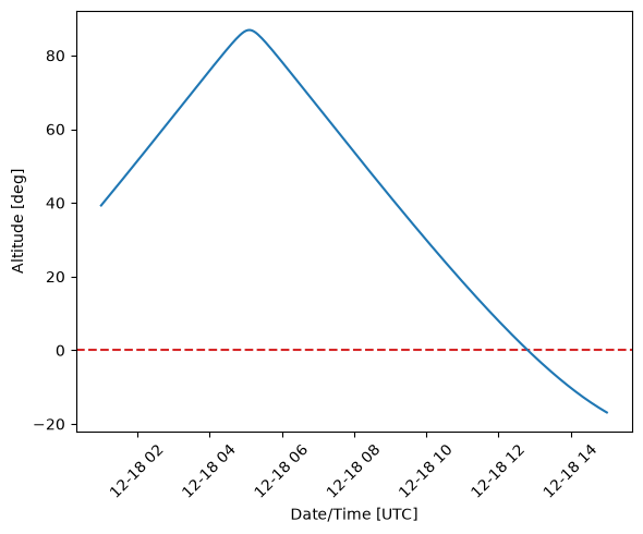
Here we can see that this open cluster reaches a high altitude above the horizon from Kitt Peak, and so it looks like it would be observable from this site. The above curve only shows the altitude trajectory for the first open cluster in our catalog, but we would like to compute the equivalent for all of the open clusters in the catalog. To do this, we have to make use of a concept that is used heavily in Numpy: array broadcasting. We have 474 open clusters and we want to evaluate the AltAz coordinates of these clusters at 256 different times.
len(open_cluster_c), len(altaz.obstime)
(474, 256)
We therefore want to produce a two-dimensional coordinate object that is indexed along one axis by the open cluster index, and along other axis by the time index. The astropy.coordinates transformation machinery supports array-like broadcasting, so we can do this by creating new, unmatched, length-1 axes on both the open clusters SkyCoord object and the AltAz frame using numpy.newaxis (doc):
open_cluster_altaz = open_cluster_c[:, np.newaxis].transform_to(altaz[np.newaxis])
Let’s now over-plot the trajectories for the first 10 open clusters in the catalog:
plt.figure(figsize=(6, 5))
plt.plot(time_grid.datetime, open_cluster_altaz[:10].alt.degree.T, marker="", alpha=0.5)
plt.axhline(0, zorder=-10, linestyle="--", color="tab:red")
plt.xlabel("Date/Time [UTC]")
plt.ylabel("Altitude [deg]")
plt.setp(plt.gca().xaxis.get_majorticklabels(), rotation=45)
plt.tight_layout()
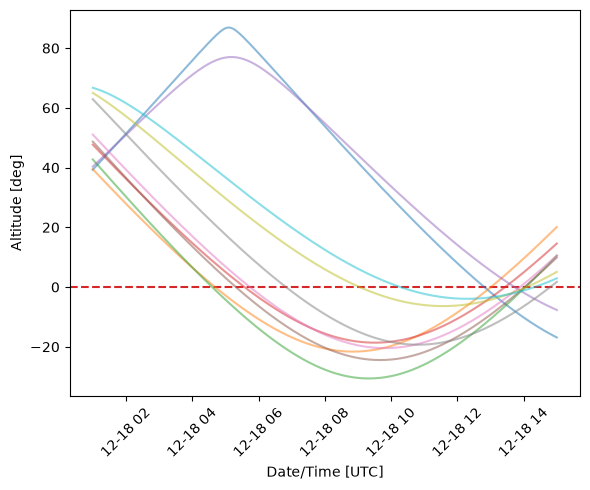
From this, we can see that only two of the clusters in this batch seem to be easily observable.
Potential Caveats#
Transformations between some reference frames require knowing more information about a source. For example, the transformation from ICRS to Galactic coordinates (as demonstrated above) amounts to a 3D rotation, but no change of origin. This transformation is therefore supported for any spherical position (with or without distance information). However, some transformations include a change of origin, and therefore require that the source data (i.e., the SkyCoord object) has defined distance information. For example, for a SkyCoord with only sky position, we can transform from the ICRS to the FK5 coordinate system:
icrs_c = coord.SkyCoord(150.4 * u.deg, -11 * u.deg)
icrs_c.transform_to(coord.FK5())
<SkyCoord (FK5: equinox=J2000.000): (ra, dec) in deg
    (150.40000705, -11.00000493)>
However, we would NOT be able to transform this position to the Galactocentric frame (docs), because this transformation involves a shift of origin from the solar system barycenter to the Galactic center:
# This cell will raise an exception and will not work (you will see a `ConvertError` exception) - this is expected!

icrs_c.transform_to(coord.Galactocentric())
---------------------------------------------------------------------------
ConvertError                              Traceback (most recent call last)
Cell In[35], line 3
      1 # This cell will raise an exception and will not work (you will see a `ConvertError` exception) - this is expected!
      2
----> 3 icrs_c.transform_to(coord.Galactocentric())

File /opt/hostedtoolcache/Python/3.12.13/x64/lib/python3.12/site-packages/astropy/coordinates/sky_coordinate.py:550, in SkyCoord.transform_to(self, frame, merge_attributes)
    546 generic_frame = GenericFrame(frame_kwargs)
    548 # Do the transformation, returning a coordinate frame of the desired
    549 # final type (not generic).
--> 550 new_coord = trans(self.frame, generic_frame)
    552 # Finally make the new SkyCoord object from the `new_coord` and
    553 # remaining frame_kwargs that are not frame_attributes in `new_coord`.
    554 for attr in set(new_coord.frame_attributes) & set(frame_kwargs.keys()):

File /opt/hostedtoolcache/Python/3.12.13/x64/lib/python3.12/site-packages/astropy/coordinates/transformations/composite.py:113, in CompositeTransform.__call__(self, fromcoord, toframe)
    110             frattrs[inter_frame_attr_nm] = attr
    112     curr_toframe = t.tosys(**frattrs)
--> 113     curr_coord = t(curr_coord, curr_toframe)
    115 # this is safe even in the case where self.transforms is empty, because
    116 # coordinate objects are immutable, so copying is not needed
    117 return curr_coord

File /opt/hostedtoolcache/Python/3.12.13/x64/lib/python3.12/site-packages/astropy/coordinates/transformations/affine.py:204, in BaseAffineTransform.__call__(self, fromcoord, toframe)
    203 def __call__(self, fromcoord, toframe):
--> 204     params = self._affine_params(fromcoord, toframe)
    205     newrep = self._apply_transform(fromcoord, *params)
    206     return toframe.realize_frame(newrep)

File /opt/hostedtoolcache/Python/3.12.13/x64/lib/python3.12/site-packages/astropy/coordinates/transformations/affine.py:258, in AffineTransform._affine_params(self, fromcoord, toframe)
    257 def _affine_params(self, fromcoord, toframe):
--> 258     return self.transform_func(fromcoord, toframe)

File /opt/hostedtoolcache/Python/3.12.13/x64/lib/python3.12/site-packages/astropy/coordinates/builtin_frames/galactocentric.py:588, in icrs_to_galactocentric(icrs_coord, galactocentric_frame)
    586 @frame_transform_graph.transform(AffineTransform, ICRS, Galactocentric)
    587 def icrs_to_galactocentric(icrs_coord, galactocentric_frame):
--> 588     _check_coord_repr_diff_types(icrs_coord)
    589     return get_matrix_vectors(galactocentric_frame)

File /opt/hostedtoolcache/Python/3.12.13/x64/lib/python3.12/site-packages/astropy/coordinates/builtin_frames/galactocentric.py:567, in _check_coord_repr_diff_types(c)
    565 def _check_coord_repr_diff_types(c):
    566     if isinstance(c.data, r.UnitSphericalRepresentation):
--> 567         raise ConvertError(
    568             "Transforming to/from a Galactocentric frame requires a 3D coordinate, e.g."
    569             " (angle, angle, distance) or (x, y, z)."
    570         )
    572     if "s" in c.data.differentials and isinstance(
    573         c.data.differentials["s"],
    574         (
   (...)    578         ),
    579     ):
    580         raise ConvertError(
    581             "Transforming to/from a Galactocentric frame requires a 3D velocity, e.g.,"
    582             " proper motion components and radial velocity."
    583         )

ConvertError: Transforming to/from a Galactocentric frame requires a 3D coordinate, e.g. (angle, angle, distance) or (x, y, z).
In this tutorial, we have introduced the key concepts that underly the astropy.coordinates framework: coordinate component formats, representations, and frames. We demonstrated how to change the representation of a SkyCoord object (e.g., Cartesian to Cylindrical). We then introduce the concept of coordinate frames and frame transformations.
Exercises#
Przybylski’s star or HD101065 is in the southern constellation of Centaurus with a right ascension of 174.4040348 degrees and a declination of -46.70953633 degrees. Create a SkyCoord object of its sky position.
If the distance to Przybylski’s star is 108.4 pc, retrieve a 3D Cartesian representation. (Hint: we did this earlier in the tutorial and it may help to create a new 3D SkyCoord object.)
Imagine it is May 2018, and you would like to take an observation of HD 101065 from Greenwich Royal Observatory. Use astropy.coordinates to figure out if you can observe the star that month (hint: use the EarthLocation class). You can use any time and date of that month for your timeframe.